10. Chapter 2: Looking at Data-Relationships#
In the previous chapters, we mainly focused on exploring the distributions of a single variable and studying statistical procedures related to that one variable or the mean of a single response variable.
Many interesting problems, however, arise when we wish to explore the relationships among two or more variables. Starting from this chapter, we will learn some graphing techniques and modeling techniques for studying the relationships among variables.
In general, if two variables have no relationship at all, we say that the variables are independent. Two variables are statistically independent if the occurrence (or value) of one does not provide any information about the occurrence (or value) of the other. In many real-world situations, true independence is rare because various factors often interrelate.
When variables are not independent, they are considered dependent; that is, knowing something about one variable gives you some information about the other. If two variables are dependent, then we say they have some kind of relationship.
In this course, we focus on the basic and most common type of relationship: the linear relationship. Among all types of relationships, we explore association and learn some basic tools to quantify it. We also touch on using linear regression modeling techniques to analyze associations and use the models as tools for prediction. Of course, there are other types of relationships among variables, such as causal relationships, which go beyond mere association.
10.1. Relationships#
Association between Variables
Two variables measured on the same cases are associated if knowing the value of one of the variables tells you something about the value of the other variable.
A response variable (dependent variable) measures an outcome of a study. An explanatory variable (independent variable) explains or causes changes in the response variable.
A description of the key characteristics of a data set that will be used to explore a relationship
between two variables should include:
Cases. Identify the cases and how many there are in the data set.
Categorical or quantitative. Classify each variable as categorical or quantitative.
Values. Identify the possible values for each variable.
Explanatory or response. If appropriate, classify each variable as explanatory or response.
Label. Identify what is used as a label variable if one is present.
10.2. Scatterplots#
The most common way to display the relationship between two quantitative variables is by using a scatterplot. It helps us to describe the form and strength of the association.
Scatterplot
A scatterplot shows the relationship between two quantitative variables measured on the same cases. The values of one variable appear on the horizontal axis, and the values of the other variable appear on the vertical axis. Each case in the data appears as the point in the plot determined by the values of both variables for that case.
Always plot the explanatory variable, if there is one, on the horizontal axis (the \(x\) axis) of a scatterplot. We usually call the explanatory variable \(x\) and the response variable \(y\). If there is no explanatory-response distinction, either variable can go on the horizontal axis. Time plots such as the one are special scatterplots where the explanatory variable \(x\) is a measure of time.
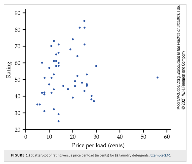
A higher price should be associated with a better product.
Instead of shape, center, and spread for distributions, we will look at form, direction, and strength for relationships.
Examining a Scatterplot
In any graph of data, look for the overall pattern and for striking deviations from that pattern.
You can describe the overall pattern of a scatterplot by the form, direction, and strength of the relationship.
When we look at it carefully, we see that it suggests a linear relationship. In other words, it may be appropriate to summarize the relationship with a straight line. To explore this possibility, we can use software to put a straight line through the data.
People’s focus on linear relationships stems from several practical and theoretical advantages.
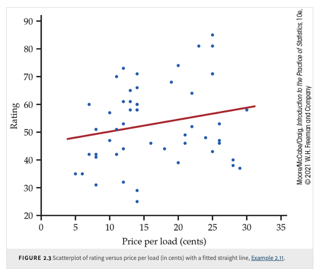
Although it is very weak, the relationship in the figure has a direction: laundry detergents that cost more have somewhat higher ratings. This is a positive association between the two variables.
Positive Association, Negative Association
Two variables are positively associated when above-average values of one tend to accompany above-average values of the other, and below-average values also tend to occur together.
Two variables are negatively associated when above-average values of one tend to accompany below-average values of the other and vice versa.
The strength of a relationship in a scatterplot is determined by how closely the points follow a clear form. The overall relationship in the figure is weak.
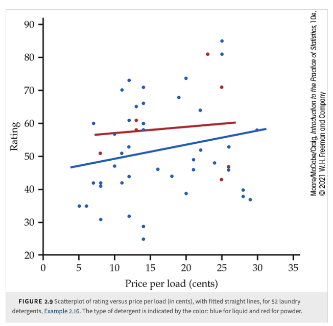
To add a categorical variable to a scatterplot, use a different plot color or symbol for each category.
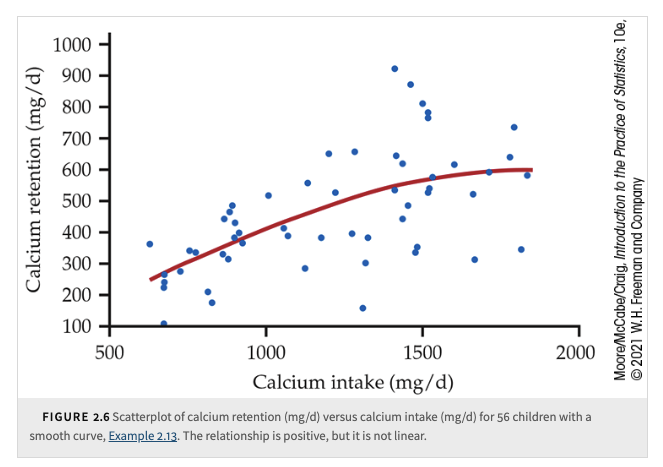
Calcium intake and retention: As calcium intake increases, the body retains more calcium, but the relationship is nonlinear—initially linear, then leveling off.
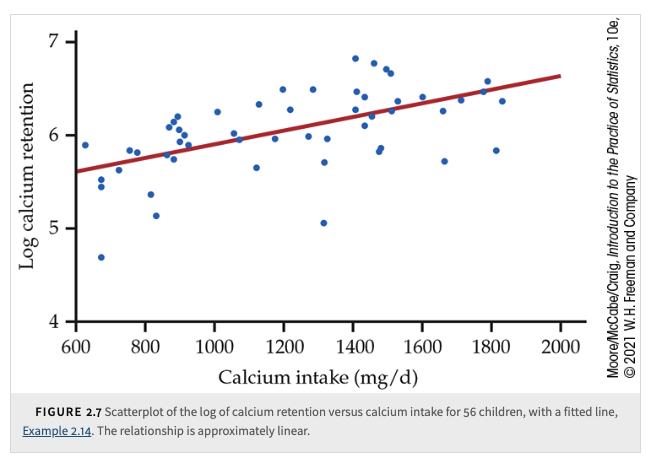
Transformations for linearity: Some curved relationships, can be made approximately linear by applying a transformation to the data.
Common use of transformations:
Help make distributions more Normal.
Convert curved relationships into more linear forms.
The Log Transformation
Purpose: Converts variables with only positive values into a more interpretable scale.
If zeros exist, replace them with a small value (e.g., half of the smallest positive value).
Logarithms in statistics:
A powerful tool for transformations.
Natural logarithms are commonly used in statistical software.
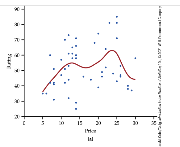
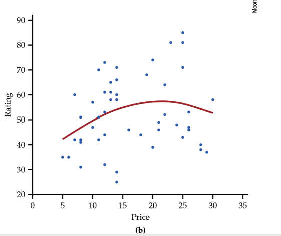
We add a smooth curve to our scatterplot to better understand the relationship between calcium retention and calcium intake. This curve helped us to see that the amount of calcium retained tends to level off as the intake increases. The method that we used to construct the curve is called smoothing.
Today, most statistical software includes options to perform the calculations needed for smoothing. The technical details vary, but the basic idea is that there is a smoothing parameter that controls the degree to which the relationship is smoothed. Here is another example.
Scatterplot of rating versus price per load (in cents), with smooth curves: (a) with a small value of the smoothing parameter; (b) with a higher value of the smoothing parameter.
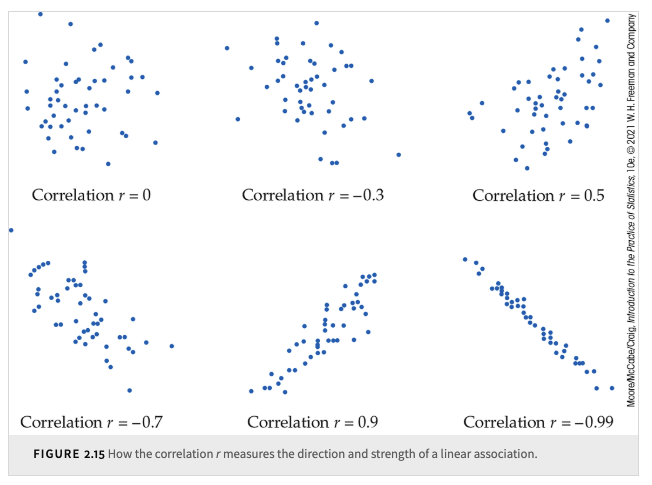
10.3. Correlation#
We have data on variables \(x\) and \(y\), two quantitative variables for \(n\) cases.
Example: Measuring height and weight of \(n\) people.
Each individual has a height \(x_i\) paired with weight \(y_i\).
These pairs are used in calculating the correlation.
Correlation
The correlation measures the direction and strength of the linear relationship between two quantitative variables.
Correlation is usually written as \(r\).
Suppose we have data on variables \(x\) and \(y\) for \(n\) individuals.
The means and standard deviations of these variables:
\(\bar{x}\) and \(s_x\) for \(x\)-values.
\(\bar{y}\) and \(s_y\) for \(y\)-values.
The correlation \(r\) is given by:
\[ r = \frac{1}{n-1} \sum \left( \frac{x_i - \bar{x}}{s_x} \right) \left( \frac{y_i - \bar{y}}{s_y} \right) \]Interpreting Correlation
Correlation values range between -1 and 1.
The two variables are said to be uncorrelated when \(r = 0\).
Values near 0 indicate a weak linear relationship.
Values near -1 or 1 indicate strong linear association.
If \(X\) and \(Y\) are independent, then \(r = 0\), but \(r = 0\) does not imply independence.
\(r = 1\) or \(r = -1\) iff \(Y = aX + b\) for some numbers \(a\) and \(b\) with \(a \neq 0\).
However, if \(|r| \ll 1\), there may still be a strong relationship between the two variables, just one that is not linear.
And even if \(|r|\) is close to 1, it may be that the relationship is really nonlinear but can be well approximated by a straight line.
Association (a high correlation) is not the same as causation.
No distinction between explanatory and response variables. No direction.
Correlation is not resistant to outliers
\(r\) is strongly affected by outliers.
Use caution when interpreting correlation in scatterplots with outliers.
Visual interpretation of \(r\) is difficult
Changing the scatterplot’s scale may mislead perception, but it does not change correlation.
Use software tools to properly assess how extreme observations influence \(r\).
A correlation based on averages is usually higher than if we used data for individuals.
Understanding the Formula
The summation sign \(\sum\) means “add these terms up.”
Though helpful in understanding correlation, it is not convenient for manual calculation.
In practice, software or a calculator should be used.
Standardization for Correlation
The formula starts by standardizing observations:
Example:
\(x\) = height (cm)
\(y\) = weight (kg)
\(\bar{x}\) and \(s_x\) are the mean and standard deviation of \(n\) heights.
Standardized Value for Height
\[ \frac{x_i - \bar{x}}{s_x} \]Z-score Interpretation
Shows how many standard deviations a value is from the mean.
Standardized values have no units.
Standardizing both variables allows for direct comparison.
Final Step
\(r\) is the average of the products of standardized height and weight values.