
9. Chapter 13: Two Way ANOVA#
One-way ANOVA examines the differences in a continuous response variable across groups defined by a single categorical factor. Two-way ANOVA extends this framework to study the effects of two categorical factors on a continuous response variable, and it also allows for the evaluation of an interaction effect between the two factors.
Why Use Two-Way ANOVA?
Multiple Factors:
When there are two independent variables (factors), two-way ANOVA can determine not only the main effect of each factor on the response but also whether the effect of one factor depends on the level of the other factor (i.e., an interaction).Efficiency and Control:
Analyzing both factors simultaneously avoids the need to perform separate one-way ANOVAs or multiple t-tests, thereby controlling the overall Type I error rate and providing a more efficient use of the data.
Example: Two-Way ANOVA with Diet and Exercise
In the one-way ANOVA example, we compared the effect of three different diets (Diet A, Diet B, Diet C) on weight loss. To extend this to a two-way ANOVA, we introduce a second factor. For instance, we might consider Exercise Level as an additional factor.
Factors and Levels
Factor 1: Diet Type
Diet A
Diet B
Diet C
Factor 2: Exercise Level
Low Exercise
High Exercise
Design
This creates a design with \(3 \times 2 = 6\) groups, as shown in the table below:
Group
Diet Type
Exercise Level
Group 1
A
Low
Group 2
A
High
Group 3
B
Low
Group 4
B
High
Group 5
C
Low
Group 6
C
High
Participants are randomly assigned to each of these 6 groups. The outcome measured (e.g., weight loss) is analyzed to see:
Main Effect of Diet:
Does the type of diet (A, B, or C) significantly affect weight loss regardless of exercise level?Main Effect of Exercise:
Does the exercise level (Low vs. High) have a significant effect on weight loss regardless of the diet?Interaction Effect:
Does the effect of the diet on weight loss depend on the exercise level? An interaction would indicate that the difference between diets might be larger (or smaller) at one exercise level compared to the other.
How Two-Way ANOVA Works
Two-way ANOVA partitions the total variability in the weight loss data into four components:
Variability due to Diet (Factor A):
Captures differences in mean weight loss among the three diets.Variability due to Exercise (Factor B):
Captures differences in mean weight loss between the two exercise levels.Variability due to the Interaction between Diet and Exercise (Interaction AB):
Captures any additional variability when the effect of diet differs between the low and high exercise groups.Residual (Error) Variability:
The variability not explained by the factors or their interaction.
Each source of variability is associated with its own sum of squares and corresponding degrees of freedom. F-statistics are computed for the main effects and interaction by comparing the mean square for each effect with the mean square of the error.
Summary
In this extended example:
One-Way ANOVA compared weight loss across three diets.
Two-Way ANOVA incorporates an additional factor (Exercise Level) to explore:
The individual effects of Diet and Exercise.
Whether there is an interaction between Diet and Exercise on weight loss.
This example shows how two-way ANOVA combines two factors to provide a more comprehensive analysis of how different treatments and conditions jointly influence the outcome.
9.1. The Two-Way ANOVA Model#
For a two-way ANOVA model, we typically construct two-way tables to either display the sample sizes in each cell or present the measured response averages (cell means) for each combination of factor levels. Here are some examples:
Controller |
Difficulty 1 |
Difficulty 2 |
Difficulty 3 |
Difficulty 4 |
Total |
|---|---|---|---|---|---|
1 |
5 |
5 |
5 |
5 |
20 |
2 |
5 |
5 |
5 |
5 |
20 |
3 |
5 |
5 |
5 |
5 |
20 |
Total |
15 |
15 |
15 |
15 |
60 |
Age group |
2010 |
2016 |
Mean |
|---|---|---|---|
Preadolescents |
108.4 |
91.1 |
99.8 |
Adolescents |
199.1 |
120.5 |
159.8 |
Adults |
121.8 |
95.2 |
108.5 |
Mean |
143.1 |
102.3 |
122.7 |
Just as we used a model to illustrate the procedure for one-way ANOVA, we similarly utilize a model to explain the procedure for two-way ANOVA. Two-way ANOVA is a statistical method used to compare population means when the populations are classified according to two factors. This approach not only assesses the individual (main) effects of each factor but also determines whether there is an interaction between the factors—that is, whether the effect of one factor depends on the level of the other.
In this section, we describe the two-way ANOVA model, explain how the total variation is partitioned, and discuss how the main effects and interactions are interpreted. We then illustrate these ideas with an example investigating differences in sugar-sweetened beverage consumption.
There are two common ways to represent the two-way ANOVA model.
The Cell Means Formulation
We can model the response in each cell directly as:
where:
\(x_{ijk}\) is the \(k\)-th observation from the cell defined by the \(i\)th level of Factor \(A\) and the \(j\)th level of Factor \(B\),
\(\mu_{ij}\) is the true mean for that cell,
\(\epsilon_{ijk}\) is the error term, assumed to be independently distributed as \(\mathcal{N}(0, \sigma^2)\).
The Decomposed Formulation
Alternatively, the cell mean \(\mu_{ij}\) can be expressed as a sum of components:
where:
\(\mu\) is the overall mean,
\(\alpha_i\) is the effect of the \(i\)th level of Factor \(A\) (with \(\sum_i \alpha_i = 0\)),
\(\beta_j\) is the effect of the \(j\)th level of Factor \(B\) (with \(\sum_j \beta_j = 0\)),
\((\alpha\beta)_{ij}\) is the interaction effect for the combination of the \(i\)th level of \(A\) and the \(j\)th level of \(B\),
\(\epsilon_{ijk}\) is as before.
These two representations are equivalent because we can define the cell mean as
Thus, the model
is simply a detailed way of writing
Design Notation:
In an \(I \times J\) ANOVA, Factor \(A\) has \(I\) levels and Factor \(B\) has \(J\) levels. Every combination of levels appears as a cell, so there are \(IJ\) cells in total.Sample Sizes:
Let \(n_{ij}\) denote the number of observations in the cell corresponding to level \(i\) of \(A\) and level \(j\) of \(B\). The total number of observations is:\[ N = \sum_{i=1}^{I} \sum_{j=1}^{J} n_{ij}. \]Group Means and Variances:
The sample mean for cell \((i, j)\) is:\[ \bar{x}_{ij} = \frac{1}{n_{ij}} \sum_{k=1}^{n_{ij}} x_{ijk}. \]A pooled estimate of the error variance \(\sigma^2\) is given by:
\[ s_p^2 = \frac{\sum_{i=1}^{I} \sum_{j=1}^{J} (n_{ij} - 1) s_{ij}^2}{\sum_{i=1}^{I} \sum_{j=1}^{J} (n_{ij} - 1)}, \]where \(s_{ij}^2\) is the sample variance in cell \((i, j)\).
Partitioning Total Variation
ANOVA partitions the total variation in the data into components attributable to the factors and their interaction, plus random error.
Total Sum of Squares (SST):
\[ SS_{Total} = \sum_{i=1}^{I} \sum_{j=1}^{J} \sum_{k=1}^{n_{ij}} \left(x_{ijk} - \bar{x}_{\cdot\cdot}\right)^2, \]where \(\bar{x}_{\cdot\cdot}\) is the overall (grand) mean.
Model Variation: This is further decomposed into:
Main Effect of Factor \(A\) (SSA): Variation among the marginal means for \(A\) (with \(I - 1\) degrees of freedom).
Main Effect of Factor \(B\) (SSB): Variation among the marginal means for \(B\) (with \(J - 1\) degrees of freedom).
Interaction Effect (SSAB): Variation due to the interaction between \(A\) and \(B\) (with \((I - 1)(J - 1)\) degrees of freedom).
Error (Within-Group) Variation (SSE):
This is the variation within each cell, with \(N - IJ\) degrees of freedom.
Thus, the total variation is partitioned as:
Main Effects
Main Effect of Factor \(A\):
This effect is assessed by comparing the marginal means of Factor \(A\) (averaging over Factor \(B\)). For example, if Factor \(A\) were “Year” (with levels 2010 and 2016), the marginal mean for each year indicates the overall effect of time.Main Effect of Factor \(B\):
This is assessed by comparing the marginal means of Factor \(B\) (averaging over Factor \(A\)). For instance, if Factor \(B\) were “Age Group,” differences in the marginal means across age groups show the effect of age.
Interaction Effect
Definition:
An interaction occurs when the effect of one factor depends on the level of the other factor. In our model, the interaction term \((\alpha\beta)_{ij}\) captures the deviation of the cell mean \(\mu_{ij}\) from what would be expected based solely on the main effects.Interpretation:
For instance, consider studying sugar-sweetened beverage consumption where:Factor \(A\) (Year): 2010 vs. 2016,
Factor \(B\) (Age Group): Preadolescents, Adolescents, Adults.
Even if the overall (marginal) effect of Year shows a reduction in consumption and the overall effect of Age Group shows differences in consumption levels, an interaction is present if the change in consumption from 2010 to 2016 is not the same for all age groups.
That is, if the effect of Year is not consistent across Age Groups, or equivalently, if the effect of Age Group is not the same in 2010 as in 2016, then an interaction exists.
The product term (Year \(\times\) Age Group) captures this mutual dependency. Note that the interaction is symmetric—stating “the effect of Year is not the same for all Age Groups” is equivalent to “the effect of Age Group is not the same for all Years.”Graphical Representation:
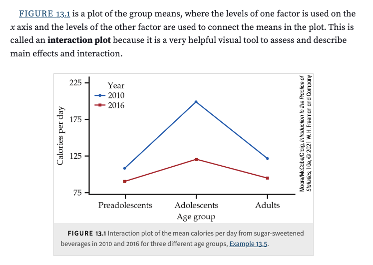
An interaction plot displays the mean response for each combination of factors. If the lines are non-parallel (i.e., the vertical gaps between the levels of one factor differ across the levels of the other), this visually indicates an interaction. The vertical difference (or “gap”) between, say, the means for 2010 and 2016 for each age group, when compared across age groups, quantifies the interaction effect.Requirement for Multiple Levels:
For an interaction to be meaningful, each factor must have at least two levels. One level typically serves as a benchmark, allowing the differences—and thus the interaction—to be observed.
Example 13.5: Investigating Differences in Sugar-Sweetened Beverage Consumption
Background:
Consumption of sugar-sweetened beverages has been linked to Type 2 diabetes and obesity. One study used data from the National Health and Nutrition Examination Survey (NHANES) with more than 57,000 individuals. Individuals were divided into three age groups:Preadolescents: 6 to 11 years,
Adolescents: 12 to 19 years,
Adults: over 19 years.
Data were collected for two years: 2010 and 2016. The table below shows the mean calories consumed per day from sugar-sweetened beverages:
Age group
2010
2016
Mean
Preadolescents
108.4
91.1
99.8
Adolescents
199.1
120.5
159.8
Adults
121.8
95.2
108.5
Mean
143.1
102.3
122.7
Marginal Means
Year Effect (Main Effect of Factor \(A\)):
Mean for 2010:
\[ \text{Mean for 2010} = \frac{108.4 + 199.1 + 121.8}{3} = 143.1 \]Mean for 2016:
\[ \text{Mean for 2016} = \frac{91.1 + 120.5 + 95.2}{3} = 102.3 \]
These are called marginal means because they are calculated at the margins (i.e., by averaging over the levels of Age Group). The overall (grand) mean is 122.7.
Age Group Effect (Main Effect of Factor \(B\)):
By averaging across the years, we obtain the marginal means for each age group:Preadolescents: 99.8 calories
Adolescents: 159.8 calories
Adults: 108.5 calories
Main Effects Observed
Effect of Year:
Overall, fewer calories were consumed in 2016 than in 2010. The reduction from 2010 to 2016 is:\[ 143.1 - 102.3 = 40.8 \text{ calories.} \]Effect of Age Group:
Adolescents consumed more calories than preadolescents and adults. For example, the increase from preadolescents to adolescents is:\[ 159.8 - 99.8 = 60 \text{ calories.} \]
Interaction Between Year and Age Group
An interaction is present when the difference between years varies across age groups. Consider the reductions from 2010 to 2016:
Adolescents:
\[ 199.1 - 120.5 = 78.6 \text{ calories.} \]Preadolescents:
\[ 108.4 - 91.1 = 17.3 \text{ calories.} \]Adults:
\[ 121.8 - 95.2 = 26.6 \text{ calories.} \]
The reduction for adolescents (78.6 calories) is much larger than for the other two groups, indicating that the effect of Year (the change from 2010 to 2016) is not the same for all Age Groups. This is the interaction effect.
Interaction Plot
An interaction plot (not shown here) would typically display:
Lines for each age group connecting the mean calories in 2010 and 2016.
Observation:
All groups show lower consumption in 2016 compared to 2010.
The vertical gap (difference between 2010 and 2016) is much larger for adolescents than for preadolescents or adults.
This non-parallelism—especially the larger gap for adolescents—visually confirms the presence of an interaction between Year and Age Group.
Two-way ANOVA relies on several key assumptions to ensure that the statistical tests are valid. The main assumptions are:
Independence:
The observations are independent of each other. This means that the data in one cell (combination of levels of Factor \(A\) and Factor \(B\)) do not influence the data in another cell.Normality:
The residuals (errors) within each cell are assumed to be normally distributed. Equivalently, the response variable in each cell is assumed to follow a Normal distribution.Homoscedasticity (Equal Variances):
The variances of the response variable are assumed to be equal across all groups (cells). This is often referred to as the assumption of homogeneity of variance.Fixed Factors (or Appropriately Random):
The factors are either fixed (levels are the only ones of interest) or, if they are random, the model and analysis must properly account for the random effects. In the standard two-way ANOVA, factors are typically considered fixed.Balanced Design (Desirable but Not Mandatory):
Although two-way ANOVA can be conducted with unequal sample sizes (unbalanced design), having equal numbers of observations in each cell (balanced design) simplifies the analysis and interpretation.
9.2. Inference for Two Way ANOVA#
Inference for two-way ANOVA naturally includes an F statistic for each of thw two main effects and the interaction. These will be summarized into the table below:
Significance Tests in Two-Way ANOVA
Significance Tests in Two-Way ANOVA
In two-way ANOVA, the overall variation in the response variable is partitioned among the main effects of two factors (commonly labeled as Factor \(A\) and Factor \(B\)), their interaction, and the residual (error) variability. There are three null hypotheses that are tested using separate \(F\) tests:
The null hypothesis for the main effect of \(A\): there is no difference among the levels of Factor \(A\).
The null hypothesis for the main effect of \(B\): there is no difference among the levels of Factor \(B\).
The null hypothesis for the interaction: the effect of one factor is the same at all levels of the other factor.
Each \(F\) statistic is computed by comparing the mean square (MS) for the source of interest with the Mean Squared Error (MSE), which is the pooled estimate of the within-group (error) variance.
The General Two-Way ANOVA Table
Below is a general format for the two-way ANOVA table:
Source
Degrees of Freedom
Sum of Squares
Mean Square
\(F\) Statistic
Factor \(A\)
\(I - 1\)
\(SSA\)
\(MSA = \dfrac{SSA}{I - 1}\)
\(F_A = \dfrac{MSA}{MSE}\)
Factor \(B\)
\(J - 1\)
\(SSB\)
\(MSB = \dfrac{SSB}{J - 1}\)
\(F_B = \dfrac{MSB}{MSE}\)
\(A \times B\) (Interaction)
\((I-1)(J-1)\)
\(SSAB\)
\(MSAB = \dfrac{SSAB}{(I-1)(J-1)}\)
\(F_{AB} = \dfrac{MSAB}{MSE}\)
Error
\(N - IJ\)
\(SSE\)
\(MSE = \dfrac{SSE}{N-IJ}\)
–
Total
\(N - 1\)
\(SST\)
–
–
Key Points:
Degrees of Freedom (DF):
For Factor \(A\): \(DF_A = I - 1\), where \(I\) is the number of levels of Factor \(A\).
For Factor \(B\): \(DF_B = J - 1\), where \(J\) is the number of levels of Factor \(B\).
For the Interaction: \(DF_{AB} = (I-1)(J-1)\).
For Error: \(DF_E = N - IJ\), where \(N\) is the total number of observations.
For Total: \(DF_{Total} = N - 1\).
Sum of Squares (SS):
These quantify the variation due to each source.\(SSA\), \(SSB\), and \(SSAB\) are calculated by comparing group or cell means with appropriate marginal or overall means.
\(SSE\) is the sum of squared deviations of individual observations from their respective cell means.
The Total Sum of Squares (\(SST\)) equals the sum of all these components:
\[ SST = SSA + SSB + SSAB + SSE. \]
Mean Square (MS):
Each MS is the Sum of Squares divided by its corresponding degrees of freedom:\[ MSA = \frac{SSA}{I-1}, \quad MSB = \frac{SSB}{J-1}, \quad MSAB = \frac{SSAB}{(I-1)(J-1)}, \quad MSE = \frac{SSE}{N-IJ}. \]\(F\) Statistic:
For each effect (main effects and interaction), the \(F\) statistic is computed as:\[ F = \frac{\text{Mean Square for the effect}}{MSE}. \]Under the null hypothesis that the effect has no influence (i.e., its contribution to the variance is zero), the \(F\) statistic follows an \(F\) distribution with numerator degrees of freedom equal to that effect’s DF and denominator degrees of freedom equal to \(DF_E\).
\(P\)-value:
The \(P\)-value is the probability that an \(F\)-distributed random variable (with the appropriate degrees of freedom) is greater than or equal to the observed \(F\) statistic. Large \(F\) values yield small \(P\)-values, leading to rejection of the null hypothesis.
Significance Level
For all hypothesis tests, including the \(F\) tests in ANOVA, a predetermined threshold called the significance level (denoted as \(\alpha\)) is set. Common choices are \(\alpha = 0.05\) or \(\alpha = 0.01\). If the \(P\)-value is less than \(\alpha\), the null hypothesis for that effect is rejected.
Summary of the Significance Tests in Two-Way ANOVA
Main Effect of Factor \(A\):
Null Hypothesis: The means across the levels of Factor \(A\) are equal.
Test Statistic: \(F_A = \frac{MSA}{MSE}\)
Decision: Reject the null if \(P\)-value \(< \alpha\).
Main Effect of Factor \(B\):
Null Hypothesis: The means across the levels of Factor \(B\) are equal.
Test Statistic: \(F_B = \frac{MSB}{MSE}\)
Decision: Reject the null if \(P\)-value \(< \alpha\).
Interaction Effect (\(A \times B\)):
Null Hypothesis: There is no interaction; the effect of one factor is consistent across the levels of the other factor.
Test Statistic: \(F_{AB} = \frac{MSAB}{MSE}\)
Decision: Reject the null if \(P\)-value \(< \alpha\).
When the variation due to the effect being tested is zero, the corresponding \(F\) statistic will be near 1, and its \(P\)-value will be large, indicating that the observed variation is consistent with random error. Conversely, a large \(F\) statistic produces a small \(P\)-value, suggesting that the observed effect is unlikely to have occurred by chance and is therefore statistically significant.
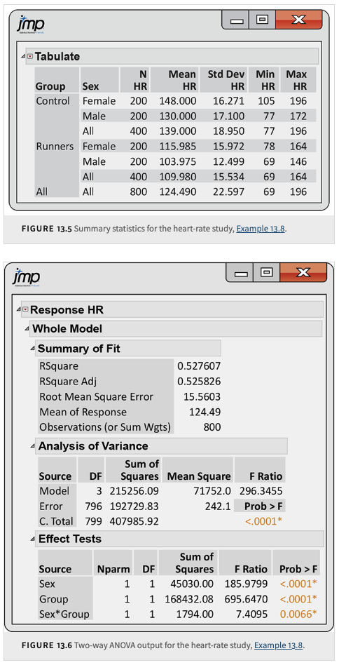
This example comes from a study of cardiovascular risk factors that compared runners (who averaged at least 15 miles per week) with a control group described as “generally sedentary.” Both men and women were included in the study. The design is a \(2 \times 2\) ANOVA with the factors Group (Control vs. Runners) and Sex (Female vs. Male). There were 200 subjects in each of the four combinations, and one of the variables measured was the heart rate (HR) after six minutes of exercise on a treadmill.
A Study of Cardiovascular Risk Factors
(1) Summary Statistics Table
This table provides descriptive statistics for each subgroup in the study. The columns are:
Group: Indicates the experimental group (e.g., “Control” or “Runners”).
Sex: The sex of the individuals in that subgroup (e.g., “Female” or “Male”).
\(N\): The number of observations (subjects) in that subgroup.
Calculation: Count the number of individuals in the subgroup.
Mean HR: The average heart rate for that subgroup.
Calculation:
\[ \text{Mean HR} = \frac{1}{N} \sum_{i=1}^{N} \text{HR}_i \]
StdDev HR: The sample standard deviation of HR in that subgroup.
Calculation:
\[ s = \sqrt{\frac{1}{N-1} \sum_{i=1}^{N} (\text{HR}_i - \text{Mean HR})^2} \]
Min HR: The minimum observed HR in the subgroup.
Max HR: The maximum observed HR in the subgroup.
For example, for the “Control Female” group with \(N=200\):
The mean HR is 148.000 (computed as the sum of all HR values for 200 individuals divided by 200).
The standard deviation is 16.271, representing how spread out the HR values are.
The minimum HR observed is 105 and the maximum is 196.
The “All” row shows the overall summary statistics for all 800 observations.
(2) Two-Way ANOVA Output
This output summarizes the results from the two-way ANOVA analysis. It is divided into two parts: the Whole Model Summary and the Analysis of Variance (ANOVA) table.
Whole Model Summary
\(R^2\): 0.527607
Meaning: Proportion of the total variability in HR that is explained by the factors (Sex, Group) and their interaction.
Calculation:
\[ R^2 = 1 - \frac{SSE}{SST} \]where \(SSE\) is the error (within-group) sum of squares and \(SST\) is the total sum of squares.
Adjusted \(R^2\): 0.525826
Meaning: \(R^2\) adjusted for the number of predictors; it penalizes the inclusion of non-significant predictors.
One Common Method:
\[ \text{Adjusted } R^2 = 1 - \frac{(1-R^2)(N-1)}{N-p-1} \]\(p\) is the number of predictors (excluding the intercept) in the model.
Root Mean Square Error (RMSE): 15.5603
Meaning: The square root of the Mean Squared Error (MSE); it provides an estimate of the standard deviation of the residuals.
Calculation:
\[ \text{RMSE} = \sqrt{MSE} = \sqrt{\frac{SSE}{df_E}} \]
Mean Response: 124.49
Meaning: The overall average HR across all observations.
Observations: 800
Meaning: The total number of data points used in the analysis.
Columns in the ANOVA Table
Source: The factor, interaction or the whole model being tested.
DF: Degrees of freedom associated with that source.
Sum of Squares (SS): The variability attributed to that source.
Mean Square (MS): The average variability per degree of freedom for that source.
Calculation:
\[ \text{MS} = \frac{\text{SS}}{\text{DF}} \]
\(F\) Ratio: The ratio of the mean square for the source to the mean square for error (MSE).
Calculation:
\[ F = \frac{MS_{\text{source}}}{MSE} \]
\(P\)-value: The probability of observing an \(F\) value as extreme as, or more extreme than, the computed \(F\) value under the null hypothesis.
Nparm: The number of parameters associated with the effect. A continuous effect has one parameter. The number of parameters for a nominal or ordinal effect is one less than its number of levels. The number of parameters for a crossed effect is the product of the number of parameters for each individual effect.
Rows in the ANOVA Table
Sex
DF: 1
Explanation: There are 2 levels of Sex (Female, Male), so \(DF = 2 - 1 = 1\).Sum of Squares: 45030.00
Explanation: Calculated by comparing the marginal means for Sex (averaged over Group) against the overall mean.Mean Square: 45030.00
Calculation: \(45030.00 / 1 = 45030.00\).\(F\) Ratio: 185.9799
Calculation: \(F = 45030.00 / MSE\), where \(MSE\) is the pooled error variance.\(P\)-value: \(<0.0001\)
Interpretation: There is a statistically significant effect of Sex on HR.
Group
DF: 1
Explanation: There are 2 groups (Control, Runners), so \(DF = 2 - 1 = 1\).Sum of Squares: 168432.08
Explanation: This measures the variability due to differences between the two groups.Mean Square: 168432.08
Calculation: \(168432.08 / 1 = 168432.08\).\(F\) Ratio: 695.6470
Calculation: \(F = 168432.08 / MSE\).\(P\)-value: \(<0.0001\)
Interpretation: There is a statistically significant effect of Group on HR, and this effect has the largest \(F\) value among the effects.
Sex*Group (Interaction)
DF: 1
Explanation: For a \(2 \times 2\) ANOVA, the interaction degrees of freedom are \((2-1) \times (2-1) = 1\).Sum of Squares: 1794.00
Explanation: This measures the variability due to the interaction between Sex and Group; that is, whether the effect of Sex on HR depends on the Group.Mean Square: 1794.00
Calculation: \(1794.00 / 1 = 1794.00\).\(F\) Ratio: 7.4095
Calculation: \(F = 1794.00 / MSE\).\(P\)-value: 0.0066
Interpretation: The interaction effect is statistically significant (with a smaller \(F\) value than the main effects).
Error
DF: 796
Explanation: The error degrees of freedom are calculated as the total number of observations minus the number of cells, i.e., \(800 - 4 = 796\).Sum of Squares: 192729.83
Explanation: This is the variability within the cells that is not explained by the factors or their interaction.Mean Square: 242.12
Calculation: \(242.12 = 192729.83 / 796\).
This is the Mean Squared Error (MSE), the pooled estimate of the error variance.
Total
DF: 799
Explanation: Total degrees of freedom is the total number of observations minus 1, i.e., \(800 - 1 = 799\).Sum of Squares: 407985.92
Explanation: This is the total variability in HR, which equals the sum of the SS for Sex, Group, their Interaction, and Error.
(3) Summary
Summary Statistics Table:
Provides descriptive measures (N, Mean, StdDev, Min, Max) for each subgroup defined by Group and Sex.Whole Model Summary:
Presents overall model diagnostics, including \(R^2\), Adjusted \(R^2\), RMSE, Mean Response, and the total number of observations.ANOVA Table:
Breaks down the total variability in HR into parts due to the main effects (Sex and Group), their interaction, and error.DF: Reflects the number of independent pieces of information for each source.
Sum of Squares: Measures the total variation attributable to each source.
Mean Square: Calculated by dividing the SS by the corresponding DF.
\(F\) Ratio: The ratio of the MS for each effect to the MSE.
\(P\)-value: Indicates the statistical significance of the effect.
Interpretation of Effects:
All three effects are statistically significant. The Group effect has the largest impact on HR, followed by the Sex effect and the interaction effect. The interaction plot (with narrow 95% confidence intervals) shows that the effect of one factor differs depending on the level of the other factor.
9.3. Mean Squares Calculations in Two Way ANOVA (Optional)#
In a two-way ANOVA, the total variation in the data is partitioned into components due to the main effects of Factor \(A\) and Factor \(B\), their interaction, and random error. Under the assumption of equal variances (homoscedasticity), the pooled error variance is estimated by the Mean Squared Error (MSE). In a balanced design—where each cell has the same number of observations \(n\)—the formulas for the sums of squares and the corresponding mean squares are as follows.
Note: For an unbalanced design (i.e., different \(n_{ij}\) across cells), the formulas are similar but involve appropriate weights (using the cell sample sizes). The degrees of freedom are adjusted accordingly.
Definitions and Notation
Let:
\(I\) = number of levels of Factor \(A\),
\(J\) = number of levels of Factor \(B\),
\(n\) = number of observations per cell (balanced design),
\(x_{ijk}\) = the \(k\)-th observation in cell \((i,j)\),
\(\bar{x}_{ij}\) = sample mean for cell \((i,j)\),
\(\bar{x}_{i\cdot}\) = marginal mean for level \(i\) of Factor \(A\) (averaged over Factor \(B\)),
\(\bar{x}_{\cdot j}\) = marginal mean for level \(j\) of Factor \(B\) (averaged over Factor \(A\)),
\(\bar{x}_{\cdot\cdot}\) = overall (grand) mean.
Sums of Squares
Sum of Squares for Factor \(A\) (SSA):
\[ SSA = Jn \sum_{i=1}^{I} (\bar{x}_{i\cdot} - \bar{x}_{\cdot\cdot})^2. \]Sum of Squares for Factor \(B\) (SSB):
\[ SSB = In \sum_{j=1}^{J} (\bar{x}_{\cdot j} - \bar{x}_{\cdot\cdot})^2. \]Sum of Squares for the Interaction between \(A\) and \(B\) (SSAB):
\[ SS_{AB} = n \sum_{i=1}^{I} \sum_{j=1}^{J} \Bigl( \bar{x}_{ij} - \bar{x}_{i\cdot} - \bar{x}_{\cdot j} + \bar{x}_{\cdot\cdot} \Bigr)^2. \]Sum of Squares for Error (SSE):
\[ SSE = \sum_{i=1}^{I} \sum_{j=1}^{J} \sum_{k=1}^{n} \Bigl( x_{ijk} - \bar{x}_{ij} \Bigr)^2. \]The total sum of squares is then given by
\[ SS_{Total} = SSA + SSB + SS_{AB} + SSE. \]Mean Squares
The mean squares are obtained by dividing each sum of squares by its associated degrees of freedom.
Mean Square for Factor \(A\) (MSA):
Degrees of freedom for Factor \(A\): \(df_A = I - 1\).
Thus,
\[ MSA = \frac{SSA}{I - 1}. \]
Mean Square for Factor \(B\) (MSB):
Degrees of freedom for Factor \(B\): \(df_B = J - 1\).
Thus,
\[ MSB = \frac{SSB}{J - 1}. \]
Mean Square for the Interaction (MSAB):
Degrees of freedom for the interaction: \(df_{AB} = (I - 1)(J - 1)\).
Thus,
\[ MS_{AB} = \frac{SS_{AB}}{(I - 1)(J - 1)}. \]
Mean Square for Error (MSE):
Degrees of freedom for Error: \(df_E = I \cdot J \cdot (n - 1)\).
Thus,
\[ MSE = \frac{SSE}{I J (n - 1)}. \]
The pooled variance (common error variance) is estimated by \(MSE\), which is then used in F-tests to compare the effects:
\(F\) for Factor \(A\): \(F_A = \dfrac{MSA}{MSE}\),
\(F\) for Factor \(B\): \(F_B = \dfrac{MSB}{MSE}\),
\(F\) for the Interaction: \(F_{AB} = \dfrac{MS_{AB}}{MSE}\).
Summary
MSA quantifies the variation among the marginal means for Factor \(A\).
MSB quantifies the variation among the marginal means for Factor \(B\).
MSAB quantifies the variation due to the interaction between Factor \(A\) and Factor \(B\).
MSE (or the pooled variance) quantifies the variation within the cells and serves as the denominator in the F-tests.
These formulas form the backbone of the two-way ANOVA analysis, allowing us to determine whether the main effects and interaction are statistically significant.