Chapter 12: One Way ANOVA

8. Chapter 12: One Way ANOVA#

In the previous chapter (Chapter 7), we learned the statistical procedure for comparing the means of two populations. Naturally, the next step is to consider what to do when there are more than two populations. For example, suppose we have three diets—Diet A, Diet B, and Diet C—administered to three independent groups drawn from different populations. The study then measures a response variable to determine whether at least one group mean differs statistically significantly from the others.

One approach is to use the two-sample procedure and perform multiple pairwise tests between the groups. In the case of three groups, this involves testing the following pairs: (Diet A, Diet B), (Diet B, Diet C), and (Diet A, Diet C). However, from our understanding of probability, each test carries a risk of a Type I error, and these errors can compound when multiple tests are conducted.

Knowing that performing multiple two-sample tests has an inherent drawback—namely, the compounded risk of Type I errors—we must pursue another approach to answer the question of whether at least one group mean differs from the others.

Recall from our study of sampling distributions that the sample mean, \(\bar{X}\), is a random variable whose variability is influenced by both the sample size \(n\) and the population standard deviation \(\sigma\). Even when drawing different samples from the same population, this inherent variability persists. In our scenario, we suspect that different groups are drawn from populations with different means (while sharing a common standard deviation). This introduces an extra layer of variability among the sample means.

To rigorously examine this question, we need a statistical procedure that formally studies the variation among multiple group means. This leads us to One-way ANOVA (Analysis of Variance). One-way ANOVA is a method used to determine whether there are any statistically significant differences among the means of three or more independent groups. Hence, we will also form a pair of hypotheses and calculate a pivotal quantity (test statistic) to run a hypothesis test to determine whether we have evidence from our dataset to reject \(H_0\). The hypotheses are as follows:

The null hypothesis in one-way ANOVA is that all group means are equal:

\[ H_0: \mu_1 = \mu_2 = \dots = \mu_k \]

The alternative hypothesis is that at least one group mean differs from the others.
The F-statistic is then compared against a critical value from the F-distribution (taking into account the degrees of freedom) to decide whether to reject the null hypothesis.

8.1. Inference for One-way ANOVA#

To concretely see how we decompose the variation of the data points in our group that leads to the variation in the sample mean (or group mean), it is best to start with a statistical model and make some assumptions. For example, consider the one-way ANOVA model:

The ANOVA model and Its Assumptions

The ANOVA model is expressed as:

\[ x_{ij} = \mu_i + \epsilon_{ij}, \]

where:

\(x_{ij}\) is the \(j\)th observation from the \(i\)th group,
\(\mu_i\) is the true (population) mean for group \(i\) — this is the systematic component (the “FIT”),
\(\epsilon_{ij}\) is the random error term — this represents the residual variation (the “RESIDUAL”).

One-way ANOVA relies on several assumptions:

Normality: The data within each group should be approximately normally distributed.
Homogeneity of Variance: The variances in different groups should be similar.
Independence: The observations must be independent of each other.
The \(\epsilon_{ij}\) are assumed to be from an \(\mathcal{N}(0, \sigma)\).

Why Assume a Common Standard Deviation?

Because sample means naturally vary due to sampling variability (which depends on both the sample size \(n\) and the underlying population standard deviation \(\sigma\)), one must assume that the populations all have the same standard deviation. This assumption, known as homogeneity of variance, is crucial. If each group had a different \(\sigma\), then the variation in the sample means would reflect not only differences in the true group means but also differences in the precision of those estimates, making it difficult to compare groups fairly.

Note

Rule for Examining Standard Deviations in ANOVA

If the largest sample standard deviation is less than twice the smallest sample standard deviation, we can use methods based on the assumption of equal standard deviations, and our results will still be approximately correct.

Decomposing Total Variation

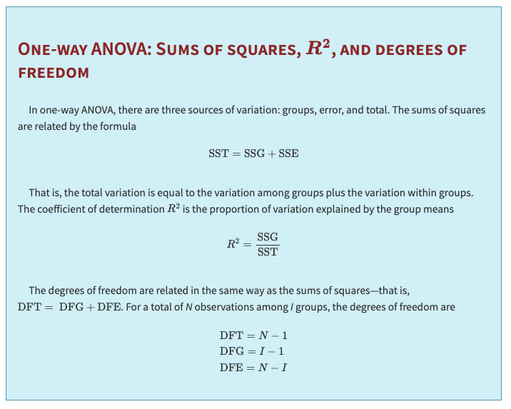
The idea behind ANOVA is that the total variation in the data can be divided into two main parts:

Between-Group Variation: Variation due to differences among the group means \(\mu_i\).
Within-Group Variation: Variation due to the random errors \(\epsilon_{ij}\) (i.e., variability within each group).

Mathematically, the total variation (often measured as the Total Sum of Squares, \(SS_{Total}\)) is given by:

\[ SS_{Total} = \sum_{i=1}^{I} \sum_{j=1}^{n_i} \left(x_{ij} - \bar{x}_{\cdot\cdot}\right)^2, \]

where \(\bar{x}_{\cdot\cdot}\) is the overall (grand) mean of all observations.

This total variation is partitioned as follows:

\[ SS_{Total} = SS_{Between} + SS_{Within}, \]

In the textbook:

\[ SST = SSG + SSE, \]

where:

Between-Group Sum of Squares (\(SS_{Between}\)):

\[ SS_{Between} = \sum_{i=1}^{I} n_i \left(\bar{x}_{i} - \bar{x}_{\cdot\cdot}\right)^2. \]

This term measures how much the group means \(\bar{x}_{i}\) differ from the overall mean. It captures the systematic differences among the groups — the variation that can be attributed to the different treatments or conditions (reflected by the \(\mu_i\)’s).
Within-Group Sum of Squares (\(SS_{Within}\)):

\[ SS_{Within} = \sum_{i=1}^{I} \sum_{j=1}^{n_i} \left(x_{ij} - \bar{x}_{i}\right)^2. \]

This term measures the variability of the observations around their respective group means, reflecting the random error \(\epsilon_{ij}\). The differences \(e_j = x_j - \bar{x}\) are the residuals and correspond to the \(\epsilon_j\) in the statistical model.

The total variation (or \(SS_{Total}\)) measures the overall spread of the individual data points around the grand mean. It tells us how much the data vary in total — a combination of:

Systematic differences among groups (if the \(\mu_i\)’s are very different, \(SS_{Between}\) is large), and
Random fluctuations within each group (if the \(\epsilon_{ij}\)’s are large, \(SS_{Within}\) is large).
These two sources of variation are independent.

Forming the F-Statistic

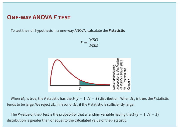
The ratio of the between-group variability to the within-group variability is computed to form the F-statistic:

\[ F = \frac{\text{Mean Square Between Groups (MSB)}}{\text{Mean Square Within Groups (MSW)}} \]

A high F-value indicates that the variability between the groups is large compared to the variability within the groups. This suggests that at least one group mean is significantly different from the others.
An F-value close to 1 indicates that the between-group variability is similar to the within-group variability, suggesting no significant differences among the group means.
Mean Square Between (MSB):

\[ MSB = \frac{SS_{Between}}{I - 1}, \]
Mean Square Within (MSW):

\[ MSW = \frac{SS_{Within}}{N - I}, \]

where \(N\) is the total number of observations across all groups.
Under the Null Hypothesis: If the null hypothesis (that all group means are equal) is true, then the expected value of both MSB and MSW is the common error variance \( \sigma^2\). Thus, under \(H_0: \mathbb{E}\left(\frac{MSB}{MSW}\right) \approx 1\).
A significantly larger F value suggests that the group means differ more than would be expected by chance, prompting rejection of the null hypothesis.

8.2. Additional Materials from the Textbook#

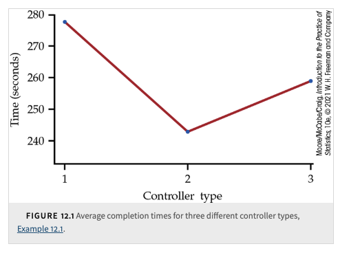
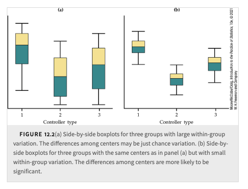
Observed Difference in Sample Mean

Is the observed difference in sample means just the result of chance variation?

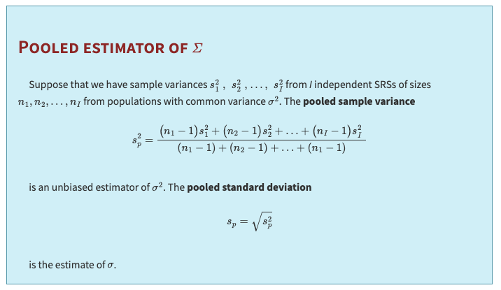
Large and Small Within-Group Variation

Pooled Estimator of \(\sigma\)

We can use the mean square for error to find \(s_p\), the pooled estimate of the parameter \(\sigma\) of our model. It is true in general that:

\[s_p^2 = \text{MSE} = \frac{\text{SSE}}{\text{DFE}}\]

In other words, the mean square for error is an estimate of the within-group variance, \(\sigma^2\). The estimate of \(\sigma\) is, therefore, the square root of this quantity. So:

\[s_p = \sqrt{\text{MSE}}\]

One-way ANOVA

One-way ANOVA F-test

JMP ANOVA Output

8.3. Supplementary Analyses Following One-Way ANOVA#

Once the overall F-test in a one-way ANOVA indicates that not all group means are equal, further analysis is needed to identify where the differences lie. Two common approaches are:

Multiple Comparisons Procedures
Contrasts

Below is an explanation of each method, why they are necessary, and their underlying logic.

Multiple Comparisons Procedures

Purpose
- Identify Specific Differences:
  While the ANOVA F-test tells you that at least one group mean is different, it does not specify which pairs of groups differ. Multiple comparisons procedures address this question by testing all (or selected) pairwise differences between group means.
Method
- Pairwise Test Statistic:
  For any two groups \(i\) and \(j\), the test statistic is computed as:
  
  \[ t_{ij} = \frac{\bar{x}_i - \bar{x}_j}{s_p \sqrt{\frac{1}{n_i} + \frac{1}{n_j}}}, \]
  
  where:
  - \(\bar{x}_i\) and \(\bar{x}_j\) are the sample means for groups \(i\) and \(j\),
  - \(n_i\) and \(n_j\) are the respective sample sizes,
  - \(s_p\) is the pooled standard deviation, assumed to estimate the common standard deviation across groups.
- Decision Rule:
  Compare \(|t_{ij}|\) with a critical value \(t^{**}\) (which is adjusted for multiple comparisons). If:
  
  \[ |t_{ij}| \geq t^{**}, \]
  
  then you conclude that the means \(\mu_i\) and \(\mu_j\) are significantly different.
Why It Is Needed
- Control of Type I Error:
  Testing many pairs increases the chance of false positives (declaring a difference when there is none). Multiple comparisons procedures use adjustments (like Bonferroni, Tukey’s HSD, etc.) to keep the overall Type I error rate at a desired level.
- Detailed Insights:
  This method provides a complete picture of which specific groups differ from each other rather than just indicating a general difference among all groups.

Contrasts

Purpose
- Test Specific Hypotheses:
  Contrasts allow you to compare specific linear combinations of group means. This is especially useful when you have predefined hypotheses or when you want to compare groups in a structured way (e.g., comparing a treatment group to a control group).
Definition
- Contrast Formula:
  A contrast is defined as:
  
  \[ \psi = \sum a_i \mu_i, \]
  
  where the coefficients \(a_i\) are chosen such that \(\sum a_i = 0\). This condition ensures that the contrast represents a meaningful comparison (for instance, the difference between two weighted averages of group means).
Confidence Interval for a Contrast
- Interval Construction:
  A confidence interval for the contrast \(\psi\) is given by:
  
  \[ c \pm t^{*} SE_c, \]
  
  where:
  - \(c\) is the estimated contrast, \(c = \sum a_i \bar{x}_i\),
  - \(SE_c\) is the standard error of the contrast estimate, \(\text{SE}_c = s_p \sqrt{\sum \frac{a_i^2}{n_i}}\),
  - \(t^{*}\) is the critical value corresponding to the desired level of confidence,
  - DFE is associated with \(s_p\).
- Hypothesis Test:
  
  To test the null hypothesis \(H_0: \psi = 0\), we use the t-statistic:
  
  \[ t = \frac{c}{\text{SE}_c} \]
Why It Is Needed
- Focused Testing:
  Contrasts allow you to test hypotheses that are more specific than “all means are equal.” For example, you might want to test whether the average of two treatment groups differs from a control group.
- Efficiency and Interpretability:
  Instead of performing all possible pairwise comparisons, contrasts let you focus on comparisons that are of practical or theoretical interest. They are particularly powerful when the comparisons were planned before the data were observed (a priori contrasts).

Chapter 12: One Way ANOVA

Contents

8. Chapter 12: One Way ANOVA#

8.1. Inference for One-way ANOVA#

8.2. Additional Materials from the Textbook#

8.3. Supplementary Analyses Following One-Way ANOVA#