Chapter 8: Inference for a Single Proportion

15. Chapter 8: Inference for a Single Proportion#

We can view Inference for a Sample Proportion as a Special Case of Inference for a Sample Mean. Below is a step-by-step comparison showing how inference for a sample proportion can be viewed as a special case of inference for a sample mean, along with the corresponding assumptions. We will walk through estimation, confidence intervals, hypothesis testing, and sample size determination.

15.1. Why Is a Sample Proportion a Special Case of a Sample Mean?#

Sample Proportion $\hat{p}$ arises naturally when each observation $X_i$ is a Bernoulli random variable (1 = “success” or 0 = “failure”) with probability $p$.
Mathematically, if $X_i \sim \mathrm{Bernoulli}(p)$, then

\[\hat{p} \;=\; \frac{1}{n}\,\sum_{i=1}^n X_i.\]

Notice that $\hat{p}$ is simply the sample mean of $\{\,X_i\}$. Hence, the usual formulas for a mean (variance, confidence intervals, test statistics) have analogues for proportions, substituting the Bernoulli variance $p(1-p)$.

15.2. Parameter of Interest#

15.2.1. General Case (Sample Mean)#

Parameter of interest: Population mean $\mu$.
Each observation $Y_i$ has mean $\mu$ and variance $\sigma^2$.
The sample mean is $\bar{Y} = \frac{1}{n}\sum_{i=1}^n Y_i$.

15.2.2. Special Case (Sample Proportion)#

Parameter of interest: True success probability $p$.
Observations $X_i \in \{0,1\}$ with $E[X_i] = p$ and $\mathrm{Var}(X_i) = p(1-p)$.
The sample proportion is $\hat{p} = \frac{1}{n}\sum_{i=1}^n X_i$.

15.3. Point Estimation#

15.3.1. Estimator#

Sample Mean: $\bar{Y}$ is the unbiased estimator of $\mu$.
Sample Proportion: $\hat{p}$ is the unbiased estimator of $p$ (equivalently, $\hat{p} = \bar{X}$ when $X_i \in \{0,1\}$).

15.3.2. Variance of the Estimator#

Sample Mean: $\mathrm{Var}(\bar{Y}) = \sigma^2 / n$.
Sample Proportion: $\mathrm{Var}(\hat{p}) = \frac{p(1-p)}{n}$.

15.4. Confidence Intervals (CIs)#

15.4.1. Large-Sample (Z-Based) CI for a Mean#

15.4.1.1. General Case#

If $\sigma$ is known (or $n$ large, so we approximate $\sigma$ by $s$), a z-interval for $\mu$ is:

\[\bar{Y} \;\pm\; z_{\alpha/2}\,\frac{\sigma}{\sqrt{n}} \quad\text{(replace $\sigma$ by $s$ if $n$ is large)}.\]

15.4.1.2. Special Case (Proportion)#

For large $n$, we use the normal approximation for $\hat{p}$:

\[\hat{p} \;\pm\; z_{\alpha/2}\,\sqrt{\frac{\hat{p}(1-\hat{p})}{n}}.\]

This is exactly the same form as the mean’s z-interval, substituting $p(1-p)$ by $\hat{p}(1-\hat{p})$. This CI is sometimes called the Wald interval for a proportion.

15.4.2. Small-Sample (T-Based) CI for a Mean#

15.4.2.1. General Case#

For smaller $n$, we often use the t-distribution:

\[\bar{Y} \;\pm\; t_{\alpha/2,\;df=n-1}\,\frac{s}{\sqrt{n}},\]

where $s$ is the sample standard deviation of $Y_i$, assuming the population is (approximately) normal.

15.4.2.2. Proportions#

Typically, we do not use a t-interval for proportions. Instead, for small $n$, one uses:

Exact binomial confidence intervals, or
Approximate intervals like the Wilson or Agresti-Coull intervals.

For large $n$, the normal (Wald) approximation is common.

15.4.3. Assumptions for Valid CI#

Mean (General):
- Random/independent sample.
- For Z-based intervals: either $\sigma$ known or large $n$ so that $\bar{Y}$ is approximately normal by the CLT.
- For T-based intervals: data from (approximately) a normal population or $n$ large enough that T is robust.
Proportion (Bernoulli):
- Random/independent Bernoulli trials.
- For the Wald (Z) interval, a common rule of thumb: $n\hat{p}\ge10$ and $n(1-\hat{p})\ge10$ (or at least 5) to ensure a decent normal approximation.

15.5. Hypothesis Testing#

15.5.1. General Framework#

A hypothesis test typically has:

\[H_0 : \theta = \theta_0 \quad \text{vs.} \quad H_a : \theta \neq \theta_0 \quad(\text{or } > \text{ or } <),\]

where $\theta$ could be $\mu$ (mean) or $p$ (proportion).

15.5.2. Z-Test (Large Samples) for a Mean#

Null Hypothesis: $H_0:\mu=\mu_0$.
Test Statistic (if $\sigma$ known or $n$ large):

\[Z = \frac{\bar{Y} - \mu_0}{\sigma/\sqrt{n}} \quad\text{(or replace $\sigma$ by $s$ if $n$ is large)}.\]

Decision: Reject $H_0$ if $|Z|$ exceeds $z_{\alpha/2}$ for a two-sided test at level $\alpha$.

15.5.3. T-Test (Small Samples) for a Mean#

If $\sigma$ is unknown and $n$ is not large, we use

\[T = \frac{\bar{Y} - \mu_0}{s/\sqrt{n}},\]

with $df = n - 1$, assuming the population is approximately normal.

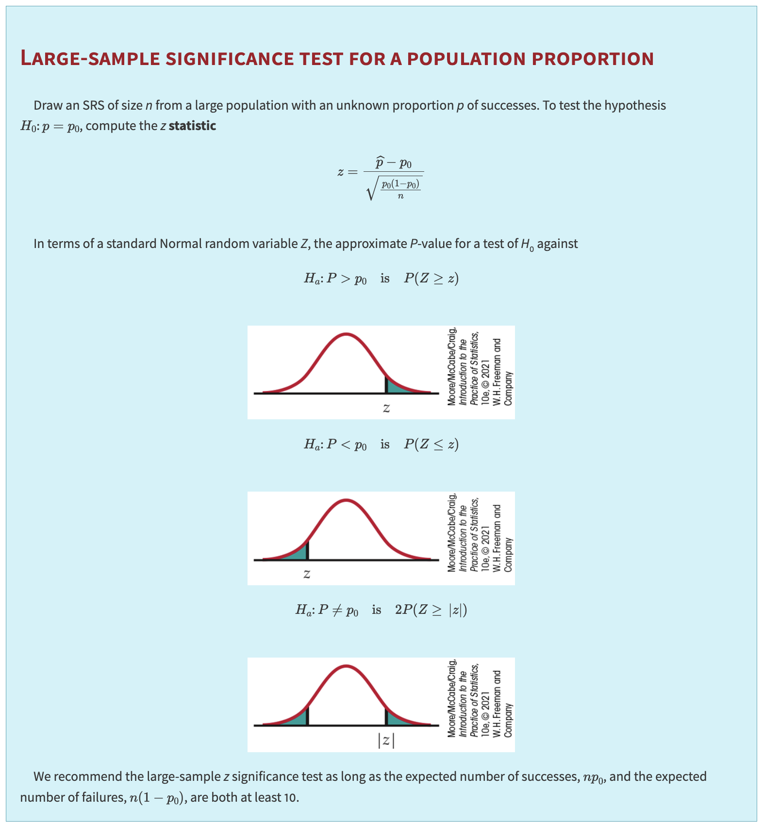
15.5.4. Z-Test for a Proportion#

Null Hypothesis: $H_0: p = p_0$.
Under $H_0$, the Bernoulli variance is $p_0(1-p_0)$.
Test Statistic:

\[Z = \frac{\hat{p} - p_0}{\sqrt{\frac{p_0(1 - p_0)}{n}}}.\]

Decision: Reject $H_0$ if $|Z| > z_{\alpha/2}$ (two-sided), or the relevant critical $z$ for one-sided tests.

15.5.5. Assumptions for Valid Testing#

Mean:
- Independent random sample.
- CLT or normality assumption for Z/T procedures.
Proportion:
- Independent Bernoulli trials.
- Large $n$ so that $\hat{p}$ is approximately normal. A rule of thumb: $n p_0 \ge 10$ and $n(1 - p_0) \ge 10$ for $H_0:p=p_0$.

15.6. Putting It All Together: Why Proportions Fit as a Special Case#

A proportion is literally the average of 0/1 outcomes.
All the formulas for means (estimation, standard error, etc.) apply, substituting $\sigma^2 = p(1-p)$.
The Central Limit Theorem applies to $\hat{p}$ just as it does to $\bar{Y}$, enabling Z-based inference for large $n$.
Key differences: the distribution assumptions (Bernoulli vs. general) and small-sample approaches (exact binomial vs. t-based).

15.7. Determining Required Sample Size for a Desired Margin of Error#

Often, we want to choose $n$ so that our confidence interval has a specified margin of error $m$.

15.7.1. For a Population Mean (Large-Sample Z-Interval)#

Assume we know (or estimate) the population standard deviation $\sigma$. The margin of error for a confidence level $C$ is

\[m = z^*\,\frac{\sigma}{\sqrt{n}},\]

where $z^*$ is the critical value (e.g., $1.96$ for 95% confidence). Solving for $n$:

\[n = \left(\frac{z^*\,\sigma}{m}\right)^2.\]

If $\sigma$ is unknown, you might use a pilot study or rough guess.

15.7.2. For a Population Proportion#

For a large-sample Z-interval for $p$, the margin of error is

\[m = z^* \,\sqrt{\frac{\hat{p}(1-\hat{p})}{n}}.\]

Before collecting data, we do not know $\hat{p}$, so we guess a value $p^*$ and solve

\[m = z^*\,\sqrt{\frac{p^*(1-p^*)}{n}} \;\;\Longrightarrow\;\; n = \left(\frac{z^*}{m}\right)^2\,p^*(1-p^*).\]

Worst-case scenario: If we want to guarantee $m$ for any $p$, set $p^* = 0.5$ (since $p(1-p)$ is maximized at 0.5). Then

\[n = \frac{1}{4}\,\Bigl(\frac{z^*}{m}\Bigr)^2.\]

15.7.3. Practical Notes#

If the actual $\hat{p}$ differs from $p^*$, the realized margin of error can be smaller or larger than planned. Using $p^*=0.5$ ensures $m$ will not be exceeded.
For means, use a reasonable guess for $\sigma$ from prior studies or a pilot sample. Overestimating $\sigma$ yields a slightly larger $n$, ensuring $m$ is not too big.
Always check that $n\hat{p}$ and $n(1-\hat{p})$ are large enough for the normal approximation. Otherwise, consider alternative (e.g. plus‐four) intervals.