
11. Chapter 2: Least Squares Regression#
In the last chapter, we have seen that we can use a straight line to study the strength of the linear relationship between two quantitative variables in the scatterplots. This line is called a regression line when one of the variables helps explain or predict the other. That is, regression describes a relationship between a response variable and an explanatory variable. It also allows us to make another type of claim about our dataset (unseen dataset), which is prediction. Because for every value on the \(x\)-axis—even if we don’t have a corresponding \(x\) value in the dataset—this regression line can still provide a corresponding \(y\) value that can be used as the prediction for the unseen \(x\) value. Prediction is a hot topic nowadays in the era of AI and Machine Learning.
Regression Line
Regression, unlike correlation, requires that we have an explanatory variable and a response variable.
A regression line is a straight line that describes how a response variable \(y\) changes as an explanatory variable \(x\) changes.
We often use a regression line to predict the value of \(y\) for a given value of \(x\).
11.1. Fitting a Line to Data#
A scatterplot displays a linear pattern, which can be summarized using a regression line.
Fitting a line means drawing a line that is as close as possible to the data points.
The fitted line provides a numerical summary of the relationship between:
Response variable \(y\)
Explanatory variable \(x\)
Straight Lines
A straight-line relationship between \(y\) and \(x\) is given by:
\[ y = b_0 + b_1x \]Interpretation of coefficients:
\(b_1\) (slope): Change in \(y\) for a one-unit increase in \(x\).
\(b_0\) (intercept): Value of \(y\) when \(x = 0\).
Software is used to compute \(b_0\) and \(b_1\) for a given dataset.
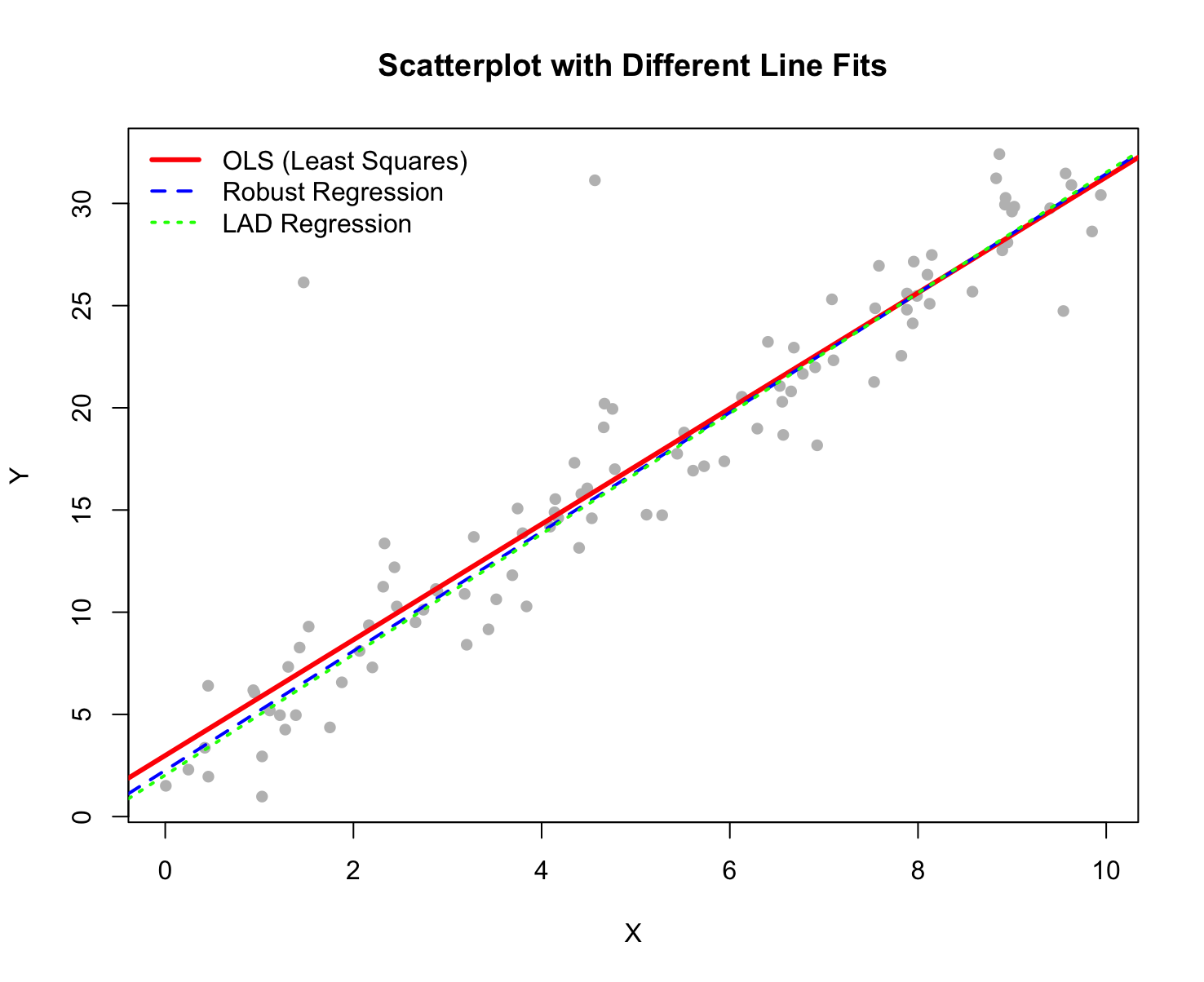
There are of course many methods to draw a line across the data points in a scatterplot. You can randomly draw a line, but one observation is that no line can pass exactly through all the data points. There are also many methods to determine the closeness between the line and the data points. Different methods will give us different pairs of values \((b_0, b_1)\). Once we obtain these parameter values, we can use the regression line as the prediction of our response variable \(y\) because we can use a particular unknown explanatory \(x\) value as the input, and it will give us the output prediction. We call this prediction \(\hat{y}\). Before we discuss the interpretation of the prediction, let’s dive a little deeper into the scatterplot to see behind the scenes how we can start from the scatterplot and obtain a Least Squares Regression Line.
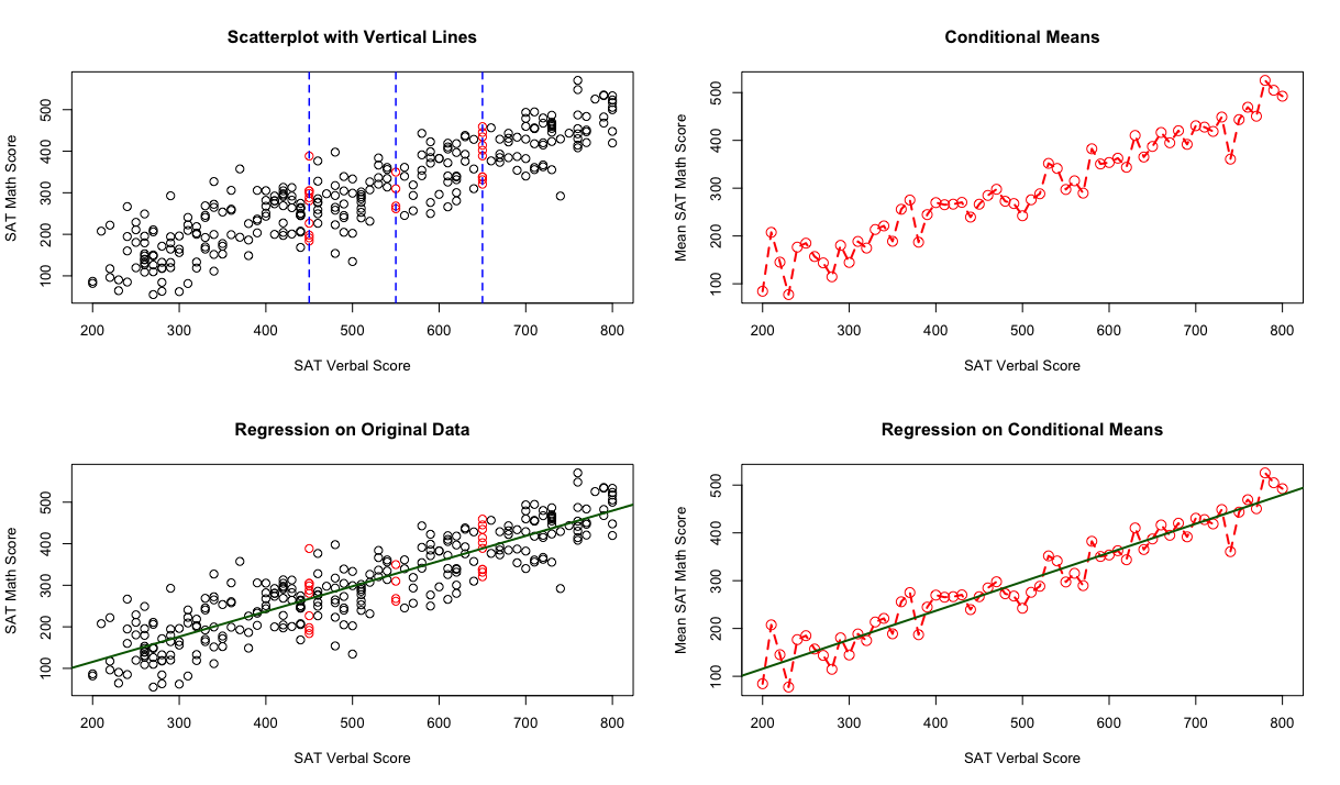
11.2. Zooming into Scatterplots#
Here we have a scatterplot (top left corner) showing many data points of the two component scores, Verbal and Math, for 200 students. The \(x\)-axis represents their Verbal scores and the \(y\)-axis represents their Math scores. As the number of data points increases, it becomes challenging to discern relationships clearly. However, we can see that for some of the data points, they share the same \(x\)-value. In these cases, the Verbal scores are identical while the Math scores differ among the students. We can focus on these data points with the same \(x\)-value, treating them as a subpopulation. By calculating the means of these points, we can better understand the relationship. We can do this for all subpopulations; these means are called the conditional means because they are conditioned on the same \(x\)-value. Then the scatterplot simplifies to the second plot, which is at the top right corner. For each \(x\)-value in this plot, we only have one \(y\)-value representing the conditional mean or average. We can interpret this as the average value of the Math score for a collection of cases at a given Verbal score.
In the third plot (bottom right corner), we fit a straight line through these conditional means, summarizing these means with a line. Finally, the last plot (bottom left corner) shows the original data points along with this straight regression line.
One thing to notice is that the regression line cannot pass through every data point and conditional mean exactly. For each data point, there is a vertical distance between the point and the line. We can calculate this distance using the formula \(e = y - \hat{y}\), which is called the residual.
11.3. Least-Squares Regression Line#
We can use a regression line to make a prediction of the response \(y\) for a specific value of the explanatory variable \(x\).
The prediction can be interpreted as:
The average value of \(y\) for a collection of cases at a given \(x\).
The best guess of \(y\) for an individual case at that particular \(x\).
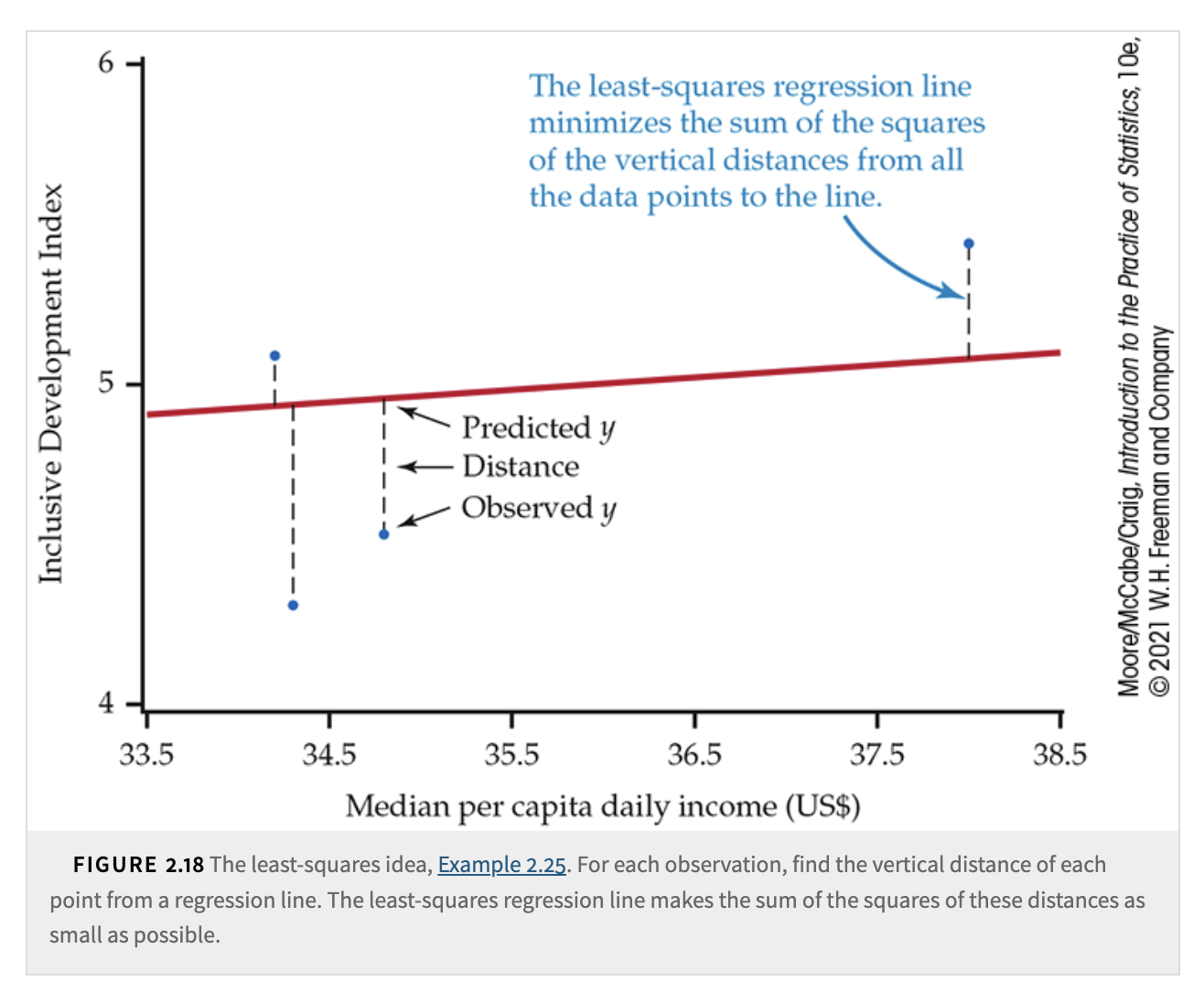
Least-Squares Regression Line
The least-squares regression line of \(y\) on \(x\) is the line that minimizes the sum of the squared vertical distances between the data points and the line.
We frequently use the terms regression line or least-squares line to describe this.
Equation of the Least-Squares Regression Line
We have data on an explanatory variable \(x\) and a response variable \(y\) for \(n\) individuals.
The means and standard deviations of the sample data:
\(\bar{x}\) and \(s_x\) for \(x\).
\(\bar{y}\) and \(s_y\) for \(y\).
The correlation coefficient between \(x\) and \(y\) is \(r\).
The equation of the least-squares regression line of \(y\) on \(x\) is:
Slope
\[ b_1 = r \frac{s_y}{s_x} \]Intercept
\[ b_0 = \bar{y} - b_1 \bar{x} \]
\(b_0\) and \(b_1\) are the regression coefficients of the least-squares equation.
11.4. Facts about Least-Squares Regression#
The use of regression to describe the relationship between a response variable and an explanatory variable is one of the most commonly encountered statistical methods. Least-squares regression is the most commonly used technique for fitting a regression line to data. Here are some key facts about least-squares regression lines.
Fact 1: Connection Between Correlation and Slope
There is a close connection between correlation and the slope of the least-squares line.
The slope is given by:\[ b_1 = r \frac{s_y}{s_x} \]This equation states that a change of 1 standard deviation in \(x\) corresponds to a change of \(r\) standard deviations in \(y\).
If \(r = 1\) or \(r = -1\), the change in \(\hat{y}\) is the same (in standard deviation units) as in \(x\).
If \(-1 \leq r \leq 1\), the change in \(\hat{y}\) is less than the change in \(x\).
As correlation weakens, the predicted \(\hat{y}\) moves less in response to changes in \(x\).
If correlation is zero, the slope of the regression line is zero.
Fact 2: The Least-Squares Regression Line Passes Through \((\bar{x}, \bar{y})\)
The least-squares regression line always passes through the point \((\bar{x}, \bar{y})\) on the graph of \(y\) against \(x\).
This means the regression line of \(y\) on \(x\) is:
A line with slope \(r \frac{s_y}{s_x}\) that passes through \((\bar{x}, \bar{y})\).
Regression can be fully described in terms of the basic measures: \(\bar{x}, s_x, \bar{y}, s_y, r\).
Fact 3: Explanatory and Response Variable Roles Matter
Regression considers distances from the line only in the \(y\)-direction.
If we switch the roles of \(x\) and \(y\), we obtain a different regression line.
11.5. Coefficient of Determination (\(R^2\)) and Square of Correlation Coefficient (\(r^2\))#
In the one-way ANOVA chapter, we have studied the coefficient of determination, \(R^2\), which represents the proportion of variance in the dependent variable \(y\) that is explained by the independent variable \(x\) in the regression model. For a simple linear regression model, where we have only one independent variable, this \(R^2\) is equal to the square of the correlation coefficient, \(r^2\), and it is also a measure of how well the regression explains the response.
Correlation \(r\) ignores the distinction between explanatory and response variables.
There is a strong connection between correlation and regression.
The slope of the least-squares regression line involves \(r\).
The numerical value of \(r\) measures the strength of a linear relationship.
\(R^2\) in Regression
The square of the correlation \(r^2\) represents the fraction of the variation in \(y\) explained by the least-squares regression of \(y\) on \(x\).
Thus, \(r^2\) is a measure of how well the regression explains the response.
For simple linear regression,
Interpretation of \(r^2\)
The square of the correlation \(r^2\) describes the variation explained by the least-squares regression.
Suppose we want to predict a new value of \(y\).
Without additional information, the best estimate is the sample mean \(\bar{y}\).
If an explanatory variable \(x\) is available, we use the regression equation:
\[ \hat{y} = b_0 + b_1 x \]
This prediction accounts for the value of \(x\).
Comparing Prediction Methods
Without \(x\):
We predict using \(\bar{y}\).
The difference between observed and predicted values is \(y - \bar{y}\).
With \(x\):
We predict using \(\hat{y}\).
The difference is \(y - \hat{y}\).
The use of \(x\) changes the error from \(y - \bar{y}\) to \(y - \hat{y}\).
We compare the sums of squares of these differences:
\[ r^2 = \frac{\sum (\hat{y} - \bar{y})^2}{\sum (y - \bar{y})^2} \]The numerator represents the variation in \(y\) explained by \(x\).
The denominator represents the total variation in \(y\).
In Chapter 11 of the textbook, where \(\hat{y}\) is based on multiple explanatory variables, we use \(R^2\) to denote the coefficient of determination.