5. Chapter 5: Sampling Distributions

In this chapter, we will begin to study statistical inference-the process of drawing conclusions about the population from the sample dataset. This involves a directional arrow from the sample dataset to the population. Typically, we are interested in either the values of population parameters or in addressing claims/statements about the population. Using information from the sample and following specific statistical procedures, we aim to:

1. Estimate population parameters.

2. Make conclusions about claims or statements related to the population.

Our goal is not merely to describe the sample dataset but to answer deeper questions such as:

• What is our best guess? - This is referred to as estimation.

• Does the data strongly contradict a proposed claim? - This is referred to as hypothesis testing.

Together, estimation and hypothesis testing form the two major pillars of frequentist[1] statistical inference.[2]

In both estimation and hypothesis testing, the process typically begins with computing a sample statistic-for example, a sample mean, a sample proportion, or a more elaborate function of the data.

For estimation, the goal is to estimate unknown population parameters (e.g., the population mean \(\mu\) or population proportion \(p\)).

• You designate a particular statistic as your estimator for the corresponding population parameter.

• When you plug in your observed data into that estimator, you obtain the estimate-a numerical result that provides your best guess for the parameter.

For hypothesis testing, the process starts with a claim or assumption about the population, called the null hypothesis (\(H_0\)). The goal is to determine if the data provide enough evidence to reject \(H_0\).

• You compute a test statistic from the sample.

• The test statistic is used to assess whether the observed data are consistent with the null hypothesis.

Details of hypothesis testing will be explored further in later chapters.

5.1. Toward Statistical Inference

Since a statistic is a central concept in the whole process, let’s revisit it and delve deeper into its meaning-like peeling an onion.

Let’s use our friend, the sample mean, as an example. In the previous chapter, we introduced the formula to calculate the sample mean \(\bar{x}\) using observed sample observations:

\[\bar{x} = \frac{x_1 + x_2 + \dots + x_n}{n}\]

This can be thought of as Stage 2 (Post-data, symbolic) in the analysis of a statistic. At this stage, you substitute the observed sample values (denoted by lowercase letters) into the function defined in Stage 1. It becomes a computed expression using the actual sample data.

Stage 1 (Pre-data): At this stage, a statistic is considered a function of random variables (denoted by uppercase letters) and is itself a random variable in theoretical probability. For the sample mean, the function is:

\[\bar{X} = \frac{X_1 + X_2 + \dots + X_n}{n}\]

The last stage, Stage 3 (A final numeric result), is where you obtain a concrete, single value from your particular dataset. The term statistic can refer to all these stages. So, it’s the same object conceptually-just viewed at three points in time:

1. Before sampling (theory): The statistic is a random variable.

2. After sampling (the formula with observed data): The statistic is computed symbolically.

3. Ultimate numeric realization: The statistic becomes a single numeric value.

In summary, a statistic evolves through these three stages as part of the analysis process.

An estimator corresponds to Stage 1, and the estimate corresponds to Stage 3. There is another term, estimand, which refers to the quantity or parameter in the population that we aim to estimate using data. The estimand represents the true but unknown value of interest, such as a mean, proportion, variance, difference, or another statistical measure describing the population.

Now that we know the three stages, let’s revisit Stage 1. At this stage, a statistic is actually a random variable, and as a random variable, it has a distribution. Imagine a thought experiment where we take one sample repeatedly, and each time, we calculate the statistic. These values form a distribution both empirically (based on repeated sampling) and hypothetically (what the statistic would look like if we had taken a different sample). This distribution is called the Sampling Distribution[3].

For a sampling distribution, we can also measure its center (mean) and its spread (variability). A statistic is an unbiased estimator of a parameter if the mean of its sampling distribution equals the true value of the population parameter. In other words, the statistic, on average, is correct.

We have already discussed the sources of bias in the sampling design section. Using random sampling can help reduce bias.

Variability describes the spread of the sampling distribution. It quantifies how much the statistic (e.g., sample mean, sample proportion) fluctuates from sample to sample. Larger samples have less variability because the sampling distribution becomes narrower as \(n\) increases. Variability usually comes from two sources:

• Sampling variability: The value of a statistic varies in repeated random sampling.

• Measurement variability: The same object could be drawn into different samples, but measurements of the object may vary.

A numerical measure of the spread of a sampling distribution is often calculated, called the margin of error. It provides bounds on the likely error when using the statistic as an estimator of a population parameter. The margin of error relates to the standard error, which is simply the standard deviation of the sampling distribution.

Ideally, we want an estimator to be both unbiased (accurate on average) and reliable (low variability).

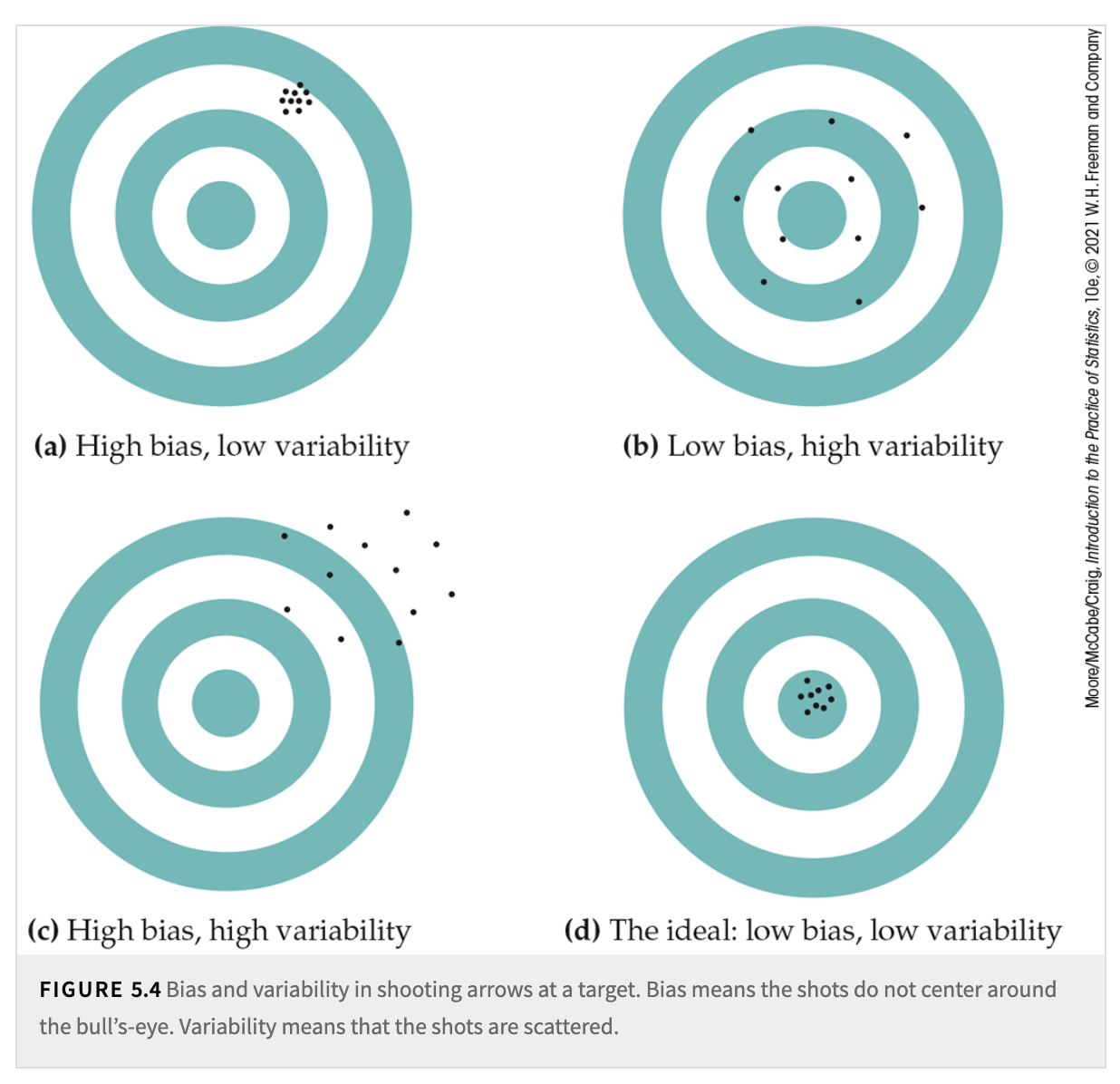
Fig. 5.1 Bias and Variability

5.2. The Sampling Distribution of a Sample Mean

From the sample mean formula presented in the previous chapter, we can see that the sample mean, \(\bar{X}\), is a sum of random variables. These random variables, \(X_1\) to \(X_n\), come from the same population distribution. If the sample size \(n\) is large, then the sampling distribution of \(\bar{X}\) is approximately normal, regardless of the shape of the population distribution[4].

This powerful result is one of the most central mathematical results in statistics, the Central Limit Theorem (CLT). In simple terms, the CLT states that the sum (or mean) of random variables follows a normal distribution as the sample size grows large.

For normal distributions, there are two parameters-mean \(\mu\) and variance \(\sigma^2\)-that govern the shape of the distribution. Using basic algebra and knowledge of probability, we can derive these two parameters for the sampling distribution.

mean of \(\bar{x}\)

If the population has mean \(\mu\), then \(\mu\) is the mean of the distribution of each observation \(X_i\). To get the mean of \(\bar{x}\), we use the rules for means of random variables. Specifically,

\[\begin{split} \mu_{\bar{x}} = \frac{1}{n} (\mu_{X_1} + \mu_{X_2} + \cdots + \mu_{X_n}) \\ = \frac{1}{n} (\mu + \mu + \cdots + \mu) \\ = \mu \end{split}\]

That is, the mean of \(\bar{x}\) is the same as the mean of the population. The sample mean \(\bar{x}\) is, therefore, an unbiased estimator of the unknown population mean \(\mu\).

variance of \(\bar{x}\)

Because the observations are independent, the addition rule for variances also applies:

\[\begin{split} \sigma_{\bar{x}}^2 = \left(\frac{1}{n}\right)^2 \left(\sigma_{X_1}^2 + \sigma_{X_2}^2 + \cdots + \sigma_{X_n}^2\right) \\ = \left(\frac{1}{n}\right)^2 \left(\sigma^2 + \sigma^2 + \cdots + \sigma^2\right) \\ = \frac{\sigma^2}{n} \end{split}\]

With \(n\) in the denominator, the variability of \(\bar{x}\) about its mean decreases as the sample size grows. Thus, a sample mean from a large sample will usually be very close to the true population mean \(\mu\).

Central Limit Theorem

Draw an SRS of size \(n\) from any population with mean \(\mu\) and finite standard deviation \(\sigma\). When \(n\) is large, the Central Limit Theorem states that the sampling distribution of the sample mean \(\bar{x}\) is approximately Normal:

\[ \bar{x} \text{ is approximately } \mathcal{N}\left(\mu, \frac{\sigma}{\sqrt{n}}\right) \]

Sampling Distribution of a Sample Mean

If a population has the \(\mathcal{N}(\mu, \sigma)\) distribution, then the sample mean \(\bar{x}\) of \(n\) independent observations has the \(\mathcal{N}(\mu, \sigma / \sqrt{n})\) distribution.

5.3. Sampling Distributions for Counts and Proportions

Before we dive into this section’s material, let us explore a new random variable and its associated distributions. The setting, with its list of requirements, is as follows. This setting appears frequently in many applications or experiments:

1. The experiment consists of a sequence of \(n\) smaller experiments called trials, where \(n\) is fixed in advance of the experiment. You can think of \(n\) data points as being drawn from the same population.

2. Each trial can result in one of the same two possible outcomes (dichotomous trials), which we generically denote by success (\(S\)) and failure (\(F\)). The assignment of the \(S\) and \(F\) labels to the two sides of the dichotomy is arbitrary. Often, we use the numerical value 1 to indicate \(S\) and 0 to indicate \(F\).

3. The trials are independent, meaning the outcome of any particular trial does not influence the outcome of any other trial.

4. The probability of success \(\mathbb{P}(S)\) is constant from trial to trial, denoted by \(p\), which represents the population proportion.

Definition 5.1 (Binomial Experiment)

An experiment that satisfies the above conditions-Condition 1, Condition 2, Condition 3, and Condition 4 (a fixed number of dichotomous, independent, and homogeneous trials)-is called a binomial experiment.

So, here we have a sample of \(n\) dichotomous data points, where each \(x_i\) in the sample takes a value of 1 or 0. The sum of these points represents the count of successes in the sample. If we calculate the sample mean \(\bar{x}\), it is simply the sample proportion. Depending on the context, we can define what constitutes a “success.”

From the results in the previous section, we know that the sampling distribution of the sample mean \(\bar{x}\) is approximately normal for large \(n\), with the following parameters:

• Mean: \(\mu_{\bar{x}} = \mu_{\text{population}} = p\)

• Standard deviation: \(\sigma_{\bar{x}} = \frac{\sigma_{\text{population}}}{\sqrt{n}} = \frac{\sqrt{p(1-p)}}{\sqrt{n}}\)

---

[1]

Besides frequentist inference, the primary alternative is Bayesian inference, where parameters are treated as random variables instead of fixed but unknown quantities.

[2]

There are other inferential frameworks and goals as well, such as prediction, model selection, and more.

[3]

The thought experiment helps us conceptualize the idea of repeated sampling. However, in practice, it is often not feasible to take repeated samples directly from the population. Instead, we can use the bootstrap algorithm to generate new samples from the available data, allowing us to approximate the sampling distribution.

[4]

The population distribution of a variable is the distribution of its values for all members of the population. The population distribution is also the probability distribution of the variable when we choose one individual at random from the population. Theoretically, all data points in the population are generated by this distribution.