13. Chapter 11: Multiple Regression

In Chapters 2 and 10, we studied methods for inference in the setting of a linear relationship between a quantitative response variable \(y\) and a single explanatory variable \(x\). In this chapter, we investigate situations in which multiple explanatory variables work together to explain, or predict, the response variable.

Here are some examples. See if you can identify the response and explanatory variables as well as determine whether each explanatory variable is quantitative or categorical.

Data for Multiple Regression

The data for a simple linear regression problem consist of \(n\) pairs of a response variable \(y\) and an explanatory variable \(x\). Because there are several explanatory variables in multiple regression, the notation needed to describe the data is more elaborate.

Each observation (or case) consists of a value for the response variable and for each of the explanatory variables. Call \(x_{ij}\) the value of the \(j\)th explanatory variable for the \(i\)th case. The data are then:

\[\begin{split}\begin{aligned} \text{Case 1:} & \quad (y_1, x_{11}, x_{12}, \ldots, x_{1p}) \\ \text{Case 2:} & \quad (y_2, x_{21}, x_{22}, \ldots, x_{2p}) \\ & \quad \vdots \\ \text{Case n:} & \quad (y_n, x_{n1}, x_{n2}, \ldots, x_{np}) \end{aligned}\end{split}\]

Here, \(n\) is the number of cases, and \(p\) is the number of explanatory variables.

Data are often entered into computer regression programs in this format. Each row is a case, and each column corresponds to a different variable.

Population Multiple Regression Equation

The simple linear regression model assumes that the mean of the response variable \(y\) depends on the explanatory variable \(x\) according to a linear equation:

\[\mu_y = \beta_0 + \beta_1 x\]

For any fixed value of \(x\), the response \(y\) varies Normally about this mean and has a standard deviation \(\sigma\) that is the same for all values of \(x\).

In the multiple regression setting, the response variable \(y\) depends on \(p\) explanatory variables, which we denote by \(x_1, x_2, \ldots, x_p\). The mean response depends on these variables according to the linear function:

\[\mu_y = \beta_0 + \beta_1 x_1 + \beta_2 x_2 + \cdots + \beta_p x_p\]

This expression is the population regression equation, and the observed values \(y\) vary about their means given by this equation.

As in simple linear regression, we can also think of this model in terms of subpopulations of responses. Each subpopulation corresponds to a particular set of values for all the explanatory variables \(x_1, x_2, \ldots, x_p\).

In each subpopulation, \(y\) varies Normally with a mean given by the population regression equation. The regression model assumes that the standard deviation \(\sigma\) of the responses is the same in all subpopulations.

13.1. The model and estimation

Multiple Linear Regression Model

Similar to simple linear regression, we combine the population regression equation and the assumptions about how the observed \(y\) vary about their means to form the multiple linear regression model. The subpopulation means describe the FIT part of our conceptual model:

\[\text{DATA} = \text{FIT} + \text{RESIDUAL}.\]

The RESIDUAL part represents how observed \(y\) deviate from their means.

We reuse the notation \(\epsilon\) for the deviation of an individual observation from its subpopulation mean. These \(\epsilon_i\) are assumed to be Normally distributed with mean 0 and the same standard deviation \(\sigma\), regardless of the \(x\) values.

MULTIPLE LINEAR REGRESSION MODEL

The multiple linear regression model is:

\[y_i = \beta_0 + \beta_1 x_{i1} + \beta_2 x_{i2} + \cdots + \beta_p x_{ip} + \epsilon_i \quad \text{for } i = 1, 2, \ldots, n,\]

where the mean response is

\[\mu_y = \beta_0 + \beta_1 x_1 + \beta_2 x_2 + \cdots + \beta_p x_p.\]

This is the population regression equation. The errors \(\epsilon_i\) are independent, Normal(0, \(\sigma\)).

The parameters of the model are the regression coefficients \(\beta_0, \beta_1, \ldots, \beta_p\) and the model standard deviation \(\sigma\).

Interpretation of Multiple Regression Coefficients

The assumption that

\[\mu_y = \beta_0 + \beta_1 x_1 + \beta_2 x_2 + \cdots + \beta_p x_p\]

links each subpopulation mean to the regression coefficients.

Key points on interpretation:

• \(\beta_0\) is the mean of \(y\) when all \(x\) variables are 0 (often not of direct interest).

• Each \(\beta_j\) (for \(j \ge 1\)) resembles a slope only if the other \(x\) variables stay fixed.

• If \(x\) variables are correlated, changes in one \(x\) may coincide with changes in others, complicating direct interpretation.

Estimation of the Multiple Regression Parameters

As in simple linear regression, we apply the least squares method to estimate the unknown coefficients. Let

\[b_0,\; b_1,\; b_2,\; \ldots,\; b_p\]

be the estimators for

\[\beta_0,\; \beta_1,\; \beta_2,\; \ldots,\; \beta_p.\]

Then, the predicted response for the \(i\)th observation is:

\[\hat{y}_i = b_0 + b_1 x_{i1} + b_2 x_{i2} + \cdots + b_p x_{ip}.\]

The residual is:

\[\begin{split}\begin{aligned} e_i &= y_i \;-\; \hat{y}_i \\ &= y_i - b_0 - b_1 x_{i1} - b_2 x_{i2} - \cdots - b_p x_{ip}. \end{aligned}\end{split}\]

The least squares estimates \((b_0, b_1, \ldots, b_p)\) minimize the sum of squared residuals:

\[\sum \Bigl(y_i - b_0 - b_1 x_{i1} - \cdots - b_p x_{ip} \Bigr)^2.\]

Estimating the Regression Standard Deviation

The actual formulas for these least-squares estimates are more involved in multiple regression, so we rely on statistical software to solve them.

We measure the variability of \(y\) around the regression equation by \(\sigma^2\). To estimate \(\sigma\), we average the squared residuals:

\[s^2 = \frac{\sum e_i^2}{\,n - p - 1\,} = \frac{\sum (y_i - \hat{y}_i)^2}{\,n - p - 1\,}, \quad s = \sqrt{s^2}.\]

ESTIMATING THE REGRESSION PARAMETERS

In multiple regression, least squares is used to estimate the population coefficients.

The model standard deviation \(\sigma\) is estimated by the regression standard error:

\[s = \sqrt{ \frac{1}{\,n - p - 1\,} \sum (y_i - \hat{y}_i)^2 }.\]

13.2. Confidence intervals, significant tests and ANOVA

Confidence Intervals & Significance Tests for Regression Coefficients

We can obtain confidence intervals and perform significance tests for each of the regression coefficients \(\beta_j\) as we did in simple linear regression. The standard errors of the \(b\)’s have more complicated formulas, but all are multiples of the estimated model standard deviation \(s\). We again rely on statistical software to do these calculations.

Confidence Intervals & Tests for \(\beta_j\)

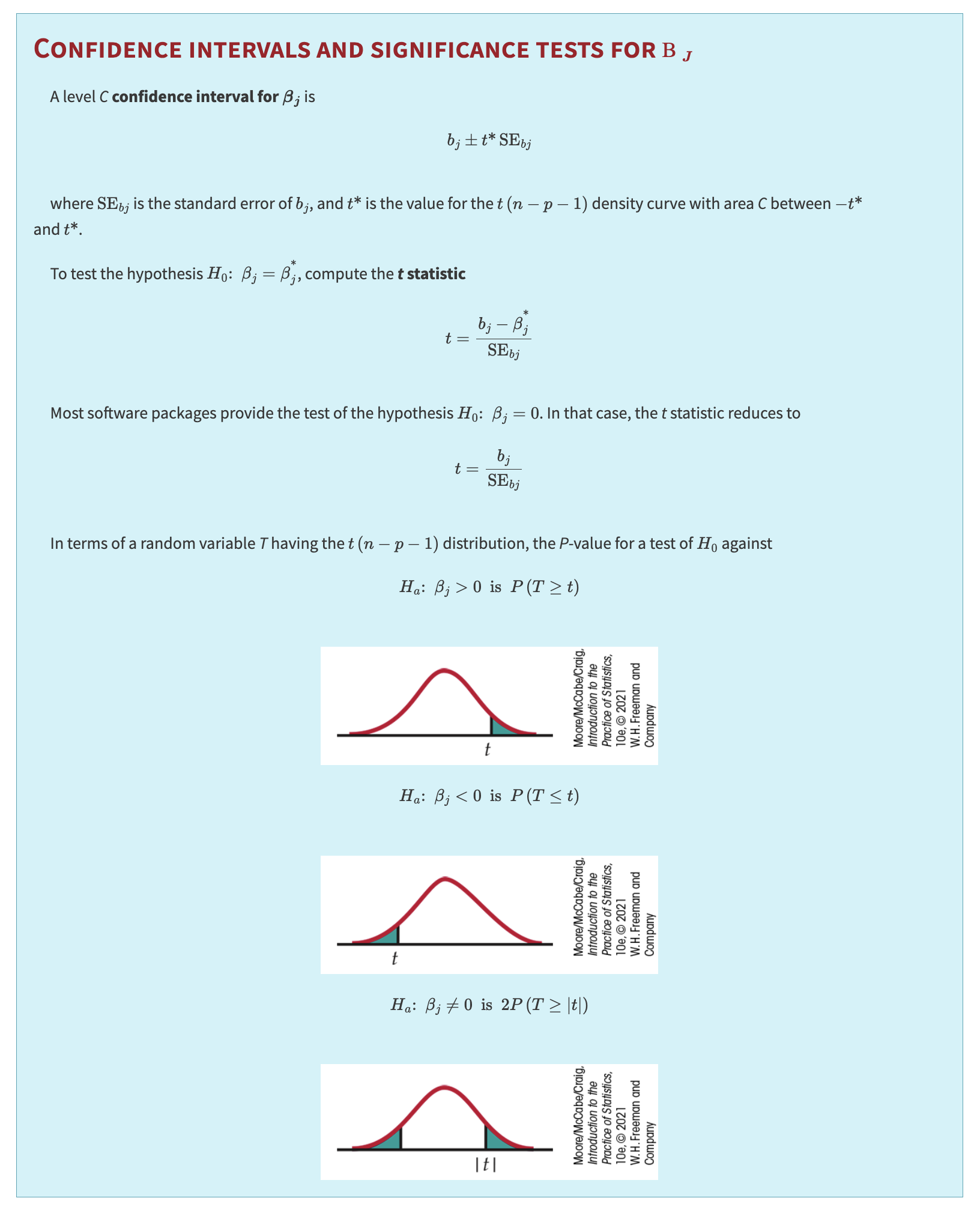
A level \(C\) confidence interval for \(\beta_j\) is

\[b_j \;\pm\; t^* \,\text{SE}_{b_j},\]

where \(\text{SE}_{b_j}\) is the standard error of \(b_j\), and \(t^*\) is the critical value from the \(t(n - p - 1)\) distribution such that the area under the curve between \(-t^*\) and \(t^*\) is \(C\).

To test the hypothesis \(H_0\!: \beta_j = \beta_j^*\), compute the test statistic:

\[t \;=\; \frac{b_j - \beta_j^*}{\text{SE}_{b_j}}.\]

Most software packages default to testing \(H_0\!: \beta_j = 0\). In that case, the test statistic reduces to:

\[t \;=\; \frac{b_j}{\text{SE}_{b_j}}.\]

If \(T\) has a \(t(n - p - 1)\) distribution, the \(P\)-value for

• \(H_a\!: \beta_j > 0 \quad\Rightarrow\quad P(T \ge t)\)

• \(H_a\!: \beta_j < 0 \quad\Rightarrow\quad P(T \le t)\)

• \(H_a\!: \beta_j \ne 0 \quad\Rightarrow\quad 2\,P(T \ge |t|)\)

Software Tips and Prediction Use

Important

Be very careful interpreting \(t\) tests and confidence intervals for individual regression coefficients.

In simple linear regression, the model \(\mu_y = \beta_0 + \beta_1 x\) implies \(H_0\!: \beta_1 = 0\) means \(x\) adds no predictive value for \(y\).

In multiple regression,

\[\mu_y = \beta_0 + \beta_1 x_1 + \beta_2 x_2 + \dots + \beta_p x_p,\]

the hypothesis \(H_0\!: \beta_1 = 0\) means \(x_1\) adds no value for predicting \(y\), given that \(x_2, \dots, x_p\) are already in the model.

In most software, the same commands that give confidence and prediction intervals in simple regression also work for multiple regression, with the only difference being that we specify multiple explanatory variables instead of just one.

ANOVA Table for Multiple Regression

In multiple regression, the \(F\) test from the ANOVA table checks whether all the regression coefficients (except the intercept) are zero.

ANOVA Table Format:

Table 13.1 ANOVA Table

Source	Degrees of Freedom	Sum of Squares	Mean Square	F
Model	\(p\)	\(\sum (\hat{y}_i - \bar{y})^2\)	SSM / DFM	MSM / MSE
Error	\(n - p - 1\)	\(\sum (y_i - \hat{y}_i)^2\)	SSE / DFE
Total	\(n - 1\)	\(\sum (y_i - \bar{y})^2\)	SST / DFT

We have

\[\text{SST} = \text{SSM} + \text{SSE}, \quad \text{DFT} = \text{DFM} + \text{DFE}.\]

The estimate of \(\sigma^2\) is again the mean square error (MSE) from the ANOVA table:

\[s^2 = \text{MSE}.\]

Interpretation of the \(F\) Statistic

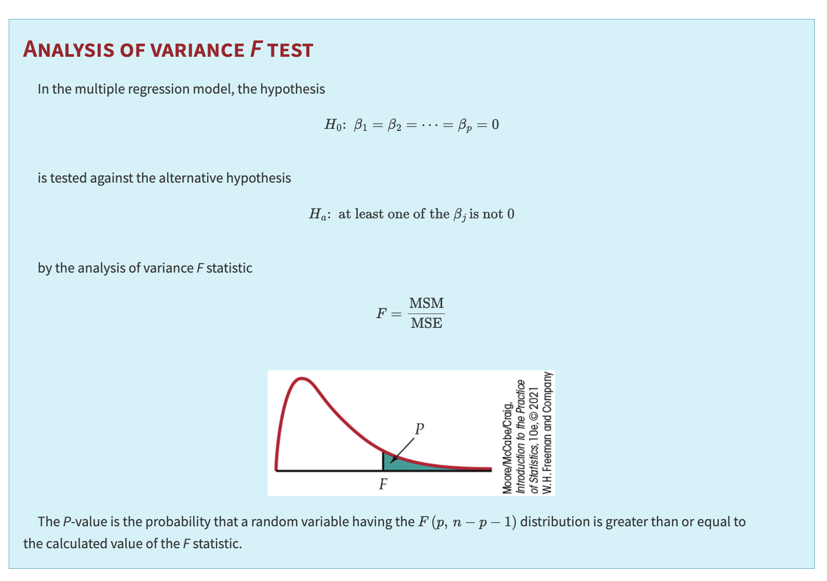
The ratio \(\text{MSM} / \text{MSE}\) is the \(F\) statistic for testing:

\[H_0\!: \beta_1 = \beta_2 = \cdots = \beta_p = 0 \quad\text{vs.}\quad H_a\!: \text{at least one of the } \beta_j \text{ is not } 0.\]

Large \(F\) values give evidence against \(H_0\). When \(H_0\) is true, \(F\) has the \(F(p,\,n - p - 1)\) distribution.

Analysis of Variance \(F\) Test (Multiple Regression)

\[H_0\!: \beta_1 = \beta_2 = \cdots = \beta_p = 0 \quad\text{vs.}\quad H_a\!: \text{at least one } \beta_j \ne 0.\]

\[F = \frac{\text{MSM}}{\text{MSE}},\]

and the \(P\)-value is \(P\bigl(F(p,\,n - p - 1)\,\ge\,F_{\text{obs}}\bigr)\).

Common Misinterpretation of the \(F\) Test

Warning

A common error in multiple regression is to assume that all coefficients are nonzero whenever \(F\) has a small \(P\)-value.

The \(F\) test provides an overall assessment of the regression model in explaining \(y\), while the individual \(t\) tests look at each variable’s importance given the others. Especially with correlated explanatory variables, a small \(P\)-value for \(F\) does not guarantee each \(\beta_j\) is statistically significant.

Squared multiple correlation \(R^2\)

For simple linear regression, we noted that the square of the sample correlation could be written as the ratio of SSM to SST and could be interpreted as the proportion of variation in \(y\) explained by \(x\). The ratio of SSM to SST is routinely calculated for multiple regression and still can be interpreted as the proportion of explained variation. The difference is that it relates to the collection of explanatory variables in the model.

The statistic \( R^2 = \frac{\text{SSM}}{\text{SST}} = \frac{\sum (\hat{y}_i - \bar{y})^2}{\sum (y_i - \bar{y})^2} \)

is the proportion of the variation of the response variable \(y\) that is explained by the explanatory variables \(x_1, x_2, \ldots, x_p\) in a multiple linear regression.

We use a capital \(R\) here to reinforce the fact that this statistic depends on a collection of explanatory variables. Often, \(R^2\) is multiplied by 100 and expressed as a percent. The square root of \(R^2\), called the multiple correlation coefficient, is the correlation between the observations \(y_i\) and the predicted values \(\hat{y}_i\). Some software provides a scatterplot of this relationship to help visualize the predictive strength of the model.

Tests