12. Chapter 10: Inference for Regression

In this chapter, we will study the inference for regression. In the previous chapter, when we had one sample—one dataset—we could plot a regression line in that scatterplot. But what if we have a different sample, a different dataset from the population? We might end up with a different regression line.

The values \(b_0\) and \(b_1\) are our estimates of the true population parameters of the linear model, which are \(\beta_0\) and \(\beta_1\). Just as we use \(\bar{x}\) to estimate \(\mu\), we need to calculate the standard errors of our estimates to quantify the sampling variability of our estimates and to conduct similar statistical inference procedures.

Understanding Uncertainty in Regression Estimates

For one scatterplot, we can have a single line given by:

\[ \hat{y} = b_0 + b_1 x \]

We use \(b_0\) to denote \(\hat{\beta}_0\), and \(b_1\) to denote \(\hat{\beta}_1\). This fitted line is fixed for that particular dataset. However, if we obtain a different dataset, which produces a different scatterplot, the pair of estimates \(b_0\) and \(b_1\) is likely to change.

The standard errors associated with \(\hat{\beta}_0\) and \(\hat{\beta}_1\) quantify the uncertainty in these estimates. They measure how much the estimates would vary if we repeated the sampling process and refitted the model each time.

• For one scatterplot, you have one fixed line with estimates \(\hat{\beta}_0\) and \(\hat{\beta}_1\).

• With a different dataset, these estimates would likely change due to sampling variability.

• The standard errors for \(\hat{\beta}_0\) and \(\hat{\beta}_1\) reflect this uncertainty and help quantify the variability of the estimated regression line across different samples.

Statistical inference is fundamentally about quantifying the uncertainty in our estimates due to sampling variability. When we draw a sample from a population, our estimates (like \(\hat{\beta}_0\) and \(\hat{\beta}_1\) in a regression model) can vary from one sample to another. Statistical inference provides tools—such as standard errors, confidence intervals, and hypothesis tests—to measure and account for this variability, allowing us to make probabilistic statements about the true population parameters despite the uncertainty inherent in any single sample. [1]

12.1. Simple Linear Regression

Having this sampling variability in mind, we can imagine observing all the data points—that is, every pair of \(x\) and \(y\) values—in the population. We also assume that \(x\) and \(y\) share a linear relationship, which can be expressed by the simple linear regression model (called “simple” because it includes only one independent variable):

Simple Linear Regression Model

• Given \(N\) observations of \((x, y)\) pairs:

  \[ (x_1, y_1), (x_2, y_2), ..., (x_N, y_N) \]

• The response variable follows:

  \[ y_i = \beta_0 + \beta_1x_i + \epsilon_i \]

• \(\beta_0\): Intercept, \(\beta_1\): Slope, \(\sigma\): Regression standard deviation.

• Error term, \(\epsilon_i \sim \mathcal{N}(0, \sigma^2)\)

• Equation: Data = Fit + Residual

• Residuals: Differences between observed and predicted \(y\) values.

Again, we assume that \(\epsilon_i \sim \mathcal{N}(0, \sigma^2)\) because not all data points lie exactly on the line; this term represents the deviation from the line. Additionally, this implies that if we condition on each \(x_i\) (as illustrated by the vertical blue dashed lines in the scatterplot from the last chapter), then by taking the average of the corresponding \(y\) values, we obtain:

\[ \mu_{y_i} = \mathbb{E}(y_i \mid x_i) = \mathbb{E}(\beta_0 + \beta_1x_i + \epsilon_i \mid x_i) = \beta_0 + \beta_1x_i + \mathbb{E}(\epsilon_i) = \beta_0 + \beta_1x_i \]

or,

\[ \mu_{y} = \beta_0 + \beta_1x \]

We can visualize this population regression line with the figure below:

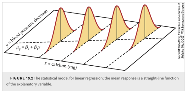
• The explanatory variable \(x\) can have multiple values (e.g., different doses of calcium supplement).

• Each value of \(x\) defines a subpopulation, assumed to have a Normally distributed response \(y\).

• The population regression line describes the mean response \(\mu_y\) as a function of \(x\).

• All subpopulations have the same spread, measured by standard deviation \(\sigma\).

• Key Assumptions:

  • The mean response \(\mu_y\) changes as \(x\) changes, forming a straight-line pattern.

  • Individual responses \(y\) vary Normally within each subpopulation.

  • Standard deviation \(\sigma\) is constant for all values of \(x\).

In reality, we cannot observe all the data points for each subpopulation; we only have a sample of data points for them. Thus, we can only obtain the estimates, \(b_0\) and \(b_1\), for the true parameters, \(\beta_0\) and \(\beta_1\), respectively.

12.2. Estimating the regression parameters

Estimating the Regression Parameters

The method of least squares presented in Chapter 2 fits a line to summarize a relationship between the observed values of an explanatory variable and a response variable. Now we want to use the least-squares regression line as a basis for inference about a population from which our observations are a sample. In that setting, the slope \(b_1\) and intercept \(b_0\) of the least-squares line

\[\hat{y} = b_0 + b_1\,x\]

estimate the slope \(\beta_1\) and the intercept \(\beta_0\) of the population regression line.

Important

This inference should only be done when the linear regression model conditions are reasonably met.

Various checks are needed, and some judgment is required. Because additional methods to check these conditions rely on first fitting the model to the data, let’s briefly review the estimation methods of Chapter 2.

Using the formulas from Chapter 2, the slope of the least-squares line is:

\[b_1 = r \,\frac{s_y}{s_x}\]

and the intercept is:

\[b_0 = \bar{y} \;-\; b_1\,\bar{x}.\]

Here, \(r\) is the correlation between the observed values of \(y\) and \(x\), \(s_y\) is the standard deviation of the sample \(y\)’s, and \(s_x\) is the standard deviation of the sample \(x\)’s.

The residuals \(e_i\) correspond to the linear regression model deviations \(\varepsilon_i\). The \(e_i\) sum to 0, and the \(\varepsilon_i\) come from a population with mean 0. Because we do not observe the \(\varepsilon_i\), we use the residuals to estimate \(\sigma\) and check the model conditions of the \(\varepsilon_i\).

\[e_i = \text{observed response} - \text{predicted response} = y_i - \hat{y}_i = y_i - b_0 - b_1\,x_i.\]

Recall also that the least-squares regression line always passes through the point \((\bar{x}, \bar{y})\). Note that if the slope \(b_1\) is 0, so is the correlation \(r\), and vice versa.

Regression Standard Error and Model Standard Deviation

To estimate \(\sigma\), which measures the variation of \(y\) about the population regression line, we look at the average squared residual (in simple linear regression). The sample of deviations is formed by the residuals \(e_i\), which stand in for the unobserved \(\varepsilon_i\).

We define:

\[s^2 = \frac{\sum e_i^2}{n - 2} = \frac{\sum (y_i - \hat{y}_i)^2}{n - 2},\]

where \(n - 2\) is the degrees of freedom for this estimate. Taking the square root of \(s^2\) gives us:

\[s = \sqrt{s^2},\]

the regression standard error. It is our estimate of the model standard deviation \(\sigma\).

Estimating the Regression Parameters

In the simple linear regression setting, we use the slope \(b_1\) and intercept \(b_0\) of the least-squares regression line to estimate the slope \(\beta_1\) and intercept \(\beta_0\) of the population regression line, respectively.

The standard deviation \(\sigma\) in the model is estimated by the regression standard error:

\[s = \sqrt{ \frac{1}{n - 2} \,\sum (y_i - \hat{y}_i)^2 }.\]

Linear Regression Model Conditions

Model Conditions vs. \(y\) and \(x\) Distributions

It is a common mistake to assess the Normality of \(y\) when checking model conditions. Even though examining the distributions of \(x\) and \(y\) can help identify outliers or influential observations, the key requirement is that the model deviations (the residuals) are approximately Normal, not necessarily \(x\) or \(y\) individually.

Linear Regression Model Conditions

To use the least-squares regression line as a basis for inference about a population, each of the following conditions should be approximately met:

• The sample is an SRS from the population.

• There is a linear relationship between \(x\) and \(y\).

• The standard deviation of the responses \(y\) about the population regression line is the same for all \(x\).

• The model deviations are Normally distributed.

In settings where the choices of \(x\) are controlled — for example, assigning subjects different milligrams of a calcium supplement — we consider the subjects to be an SRS from the population, and that they are randomly assigned to the different choices of \(x\). In other words, the \(y\)’s for each value of \(x\) are an SRS from its subpopulation.

Provided our check of conditions gives no reason to question the use of the simple linear regression model, we can proceed to inference about:

• The slope \(\beta_1\) and the intercept \(\beta_0\) of the population regression line.

• The mean response \(\mu_y\) for a given value of \(x\).

• An individual future response \(y\) for a given value of \(x\).

12.3. Confidence intervals and significant tests

Confidence Intervals and Significance Tests

Chapter 7 presented confidence intervals and significance tests for means and differences in means. In each case, inference rested on the standard errors of estimates and on \(t\) distributions. Inference in simple linear regression is similar in principle. For example, the confidence intervals have the form:

\[\text{estimate} \;\pm\; t^* \cdot \text{SE}_{\text{estimate}},\]

where \(t^*\) is a critical point of a \(t\) distribution. It is only the formulas for the estimate and standard error that are different.

As a consequence of the model assumptions about the deviations \(\varepsilon_i\), the sampling distributions of \(b_0\) and \(b_1\) are Normally distributed with means \(\beta_0\) and \(\beta_1\) and standard deviations that are multiples of \(\sigma\), the model parameter that describes the variability about the true regression line. In fact, even if the \(\varepsilon_i\) are not Normally distributed, a general form of the central limit theorem tells us that the distributions of \(b_0\) and \(b_1\) will be approximately Normal.

Because we do not know \(\sigma\), we use the estimated model standard deviation \(s\), which measures the variability of the data about the least-squares line. When we do this, we again move from the Normal distribution to \(t\) distributions but now with degrees of freedom \(n - 2\), the degrees of freedom of \(s\). We give formulas for the standard errors \(\text{SE}_{b_1}\) and \(\text{SE}_{b_0}\) in Section 10.2 of the textbook.

Inference for the Regression Slope

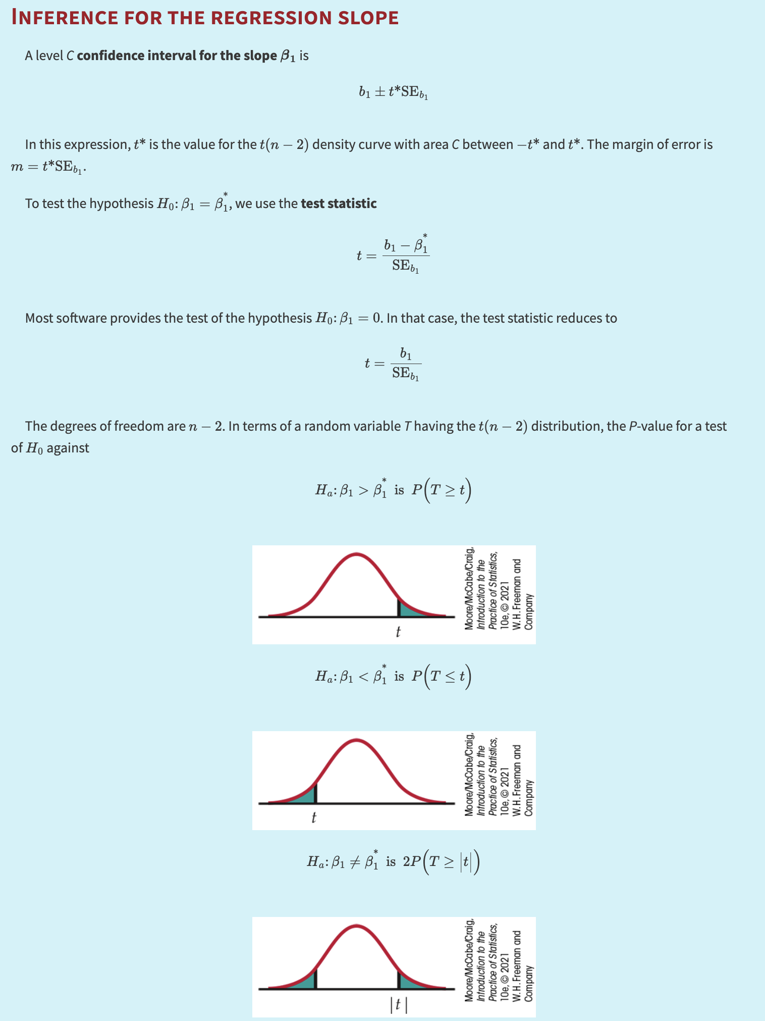
INFERENCE FOR THE REGRESSION SLOPE

A level \(C\) confidence interval for the slope \(\beta_1\) is:

\[b_1 \;\pm\; t^* \cdot \text{SE}_{b_1},\]

where \(t^*\) is the value for the \(t(n - 2)\) density curve with area \(C\) between \(-t^*\) and \(t^*\). The margin of error is \(m = t^* \cdot \text{SE}_{b_1}\).

To test the hypothesis \(H_0\!: \beta_1 = \beta_1^*\), we use the test statistic:

\[t = \frac{b_1 - \beta_1^*}{\text{SE}_{b_1}}.\]

If \(H_0\!: \beta_1 = 0\), then the test statistic reduces to:

\[t = \frac{b_1}{\text{SE}_{b_1}}.\]

With degrees of freedom \(n - 2\), the \(P\)-value for the hypothesis depends on the alternative:

\[\begin{split}\begin{aligned} H_a: \beta_1 > \beta_1^* & \;\Rightarrow\; P(T \ge t), \\ H_a: \beta_1 < \beta_1^* & \;\Rightarrow\; P(T \le t), \\ H_a: \beta_1 \ne \beta_1^* & \;\Rightarrow\; 2\,P(T \ge |t|). \end{aligned}\end{split}\]

Testing the Intercept and the Slope

Formulas for confidence intervals and significance tests for the intercept \(\beta_0\) are exactly the same, replacing \(b_1\) and \(\text{SE}_{b_1}\) by \(b_0\) and its standard error \(\text{SE}_{b_0}\).

Although computer outputs often include a test of \(H_0: \beta_0 = 0\), this usually has little practical value. From the equation \(\mu_y = \beta_0 + \beta_1 x\), we see that \(\beta_0\) is the mean response when \(x = 0\), which is often not meaningful.

The test of \(H_0: \beta_1 = 0\) is more useful. When \(\beta_1 = 0\), the model becomes:

\[\mu_y = \beta_0.\]

This implies that the mean of \(y\) does not vary with \(x\). All \(y\) values come from a population with mean \(\beta_0\) (estimated by \(\bar{y}\)), and there is no straight-line relationship between \(x\) and \(y\).

Interpreting P-values:

Note, a large \(t\) value however, that this is not the same as concluding that we have found a strong linear relationship. As seen in Figure 10.3 in the textbook, there can be substantial scatter.

Important

A very small \(P\)-value for the significance test for a zero slope does not necessarily imply that we have found a strong relationship.

A confidence interval provides more information. In software, these intervals may be optional and must be requested. They can also be constructed by hand.

Confidence Intervals for Mean Response

Besides slope and intercept, we may want to use the regression line to estimate the mean response \(y\) at a specific \(x = x^*\). The mean of the response is:

\[\mu_y = \beta_0 + \beta_1\,x^*.\]

The estimate is:

\[\hat{\mu}_y = b_0 + b_1\,x^*.\]

CONFIDENCE INTERVAL FOR A MEAN RESPONSE

\[\hat{\mu}_y \;\pm\; t^* \cdot \text{SE}_{\hat{\mu}_y},\]

where \(t^*\) is from the \(t(n - 2)\) distribution and \(m = t^* \cdot \text{SE}_{\hat{\mu}_y}\).

Prediction Intervals

To predict an individual observation \(y\) for \(x = x^*\), we again use:

\[\hat{y} = b_0 + b_1\,x^*.\]

This looks like the same formula as for \(\hat{\mu}_y\), but here it predicts a single future value. We use different notation to emphasize:

• \(\hat{y}\) for future value,

• \(\hat{\mu}_y\) for population mean.

For example, predicted BMI \(= 23.7\ \text{kg/m}^2\). But a useful prediction also needs a margin of error.

A prediction interval is used to estimate where a future observation will fall. It is wider than the confidence interval because it includes both:

• variability around the regression line,

• variability of future observations.

Repeat:

• Sample \(n\) points \((x_i, y_i)\) and one more \((x^*, y)\).

• Construct a 95% prediction interval for \(y\) using \(x^*\).

Prediction Interval for a Future Observation:

PREDICTION INTERVAL FOR A FUTURE OBSERVATION

A level \(C\) prediction interval for a future observation \(y\) from the subpopulation corresponding to \(x^*\) is:

\[\hat{y} \;\pm\; t^* \cdot \text{SE}_{\hat{y}},\]

where \(t^*\) comes from \(t(n - 2)\) with area \(C\) between \(-t^*\) and \(t^*\).
The margin of error is \(m = t^* \cdot \text{SE}_{\hat{y}}\).

Then, 95% of such intervals will capture the true \(y\) for a future observation. The formula for \(\text{SE}_{\hat{y}}\) includes both the uncertainty of estimating the line and variability around the mean.

12.4. More detail about simple linear regression

Analysis of Variance for Regression

The usual computer output for regression includes an additional block of calculations labeled “ANOVA” or “Analysis of Variance.”
Analysis of variance (often abbreviated ANOVA) refers to statistical methods that break down the total variation in the data into pieces that correspond to different sources of variation. It aligns with the conceptual framework:

\[\text{DATA = FIT + RESIDUAL.}\]

The total variation in the response \(y\) is expressed by the deviations \(y_i - \bar{y}\). If these deviations were all zero, then all observations would be the same, implying no variation in \(y\). When there is variation (i.e., \(y_i\) are not all equal to \(\bar{y}\)), the linear regression model identifies two sources for this variation:

1. As the explanatory variable \(x\) changes, the mean response changes with it along the regression line. The fitted value \(\hat{y}_i\) estimates the mean response for each \(x_i\). The differences \(\hat{y}_i - \bar{y}\) reflect the variation in mean response due to differences in the \(x_i\).

2. Individual observations vary about their subpopulation mean, captured by the residuals \(y_i - \hat{y}_i\) that record how much the actual observations scatter about the fitted line.

Hence, each deviation \(y_i - \bar{y}\) can be split into:

\[(y_i - \bar{y}) = (\hat{y}_i - \bar{y}) \;+\; (y_i - \hat{y}_i),\]

conveying the idea DATA = FIT + RESIDUAL.

Several Ways to Measure Variation:

We often measure variation by taking an average of squared deviations. By squaring each of the three deviations (data, fit, residual) and summing across \(n\) observations, we get:

\[\sum (y_i - \bar{y})^2 \;=\; \sum (\hat{y}_i - \bar{y})^2 \;+\; \sum (y_i - \hat{y}_i)^2.\]

We rewrite it as:

\[\text{SST} \;=\; \text{SSM} \;+\; \text{SSE},\]

where

\[\text{SST} = \sum (y_i - \bar{y})^2, \quad \text{SSM} = \sum (\hat{y}_i - \bar{y})^2, \quad \text{SSE} = \sum (y_i - \hat{y}_i)^2.\]

• SST (Total Sum of Squares) is the total variation in \(y\).

• SSM (Model Sum of Squares) measures the variation along the regression line (explained by \(x\)).

• SSE (Error Sum of Squares) is the residual or unexplained variation.

If \(b_1 = 0\), then SSM \(= 0\) and SST \(=\) SSE.

When \(H_0\!: \beta_1 = 0\) holds, there is no subpopulation structure and all \(y_i\) come from a single population with mean \(\mu_y\) (no linear dependence on \(x\)).

Sums of Squares, Degrees of Freedom, and Mean Squares:

SUMS OF SQUARES, DEGREES OF FREEDOM, AND MEAN SQUARES

Sums of squares represent the total variation present in the responses. We have:

\[\text{SST = SSM + SSE}\]

with corresponding degrees of freedom:

\[\text{DFT = DFM + DFE}.\]

To calculate mean squares:

\[\text{MS} = \frac{\text{sum of squares}}{\text{degrees of freedom}}.\]

From Section 2.4, recall that \(r^2\) is the fraction of the variation in \(y\) explained by the least-squares regression:

\[r^2 = \frac{\text{SSM}}{\text{SST}} = \frac{\sum (\hat{y}_i - \bar{y})^2}{\sum (y_i - \bar{y})^2}.\]

Hence, \(r^2\) is the proportion of explained variation in \(y\).

Mean Squares and MSE:

Recall that the sample variance for \(y\) is:

\[s_y^2 = \frac{\sum (y_i - \bar{y})^2}{n - 1},\]

which uses SST in the numerator and total degrees of freedom \(\text{DFT} = n - 1\). Meanwhile, the degrees of freedom break down as:

\[\text{DFT} = \text{DFM} + \text{DFE}.\]

For regression with one explanatory variable, \(\text{DFM} = 1\), so \(\text{DFE} = n - 2\). In general:

\[\text{MS} = \frac{\text{sum of squares}}{\text{degrees of freedom}} \quad\text{and}\quad \text{MSE} = s^2 = \frac{\sum (y_i - \hat{y}_i)^2}{n - 2}.\]

The ANOVA \(F\) Test

The null hypothesis \(H_0\!: \beta_1 = 0\) can be tested using the \(F\) statistic:

\[F = \frac{\text{MSM}}{\text{MSE}}.\]

If \(H_0\) is true, \(F\) follows an \(F\) distribution with 1 numerator df and \(n - 2\) denominator df. \(F\) distributions are right-skewed, indexed by \(F(j, k)\) where \(j\) is numerator df and \(k\) is denominator df. The peak is near 1.

Critical Values and Tables:

Figure 10.14 illustrates the density curve for \(F(9, 10)\).

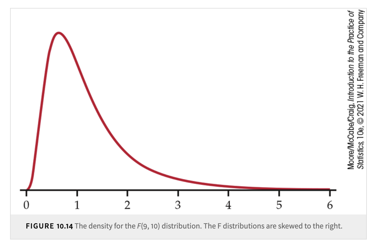
If software does not provide \(P\)-values, you can consult tables of critical \(F\) values (for example, \(p = 0.100, 0.050, 0.025, 0.010, 0.001\)). In simple linear regression, the numerator degrees of freedom = 1, and denominator df = \(n - 2\).

ANOVA Table Structure:

Table 12.1 Analysis of Variance

Source	Degrees of Freedom	Sum of Squares	Mean Square	\(F\)
Model	1	\(\sum (\hat{y}_i - \bar{y})^2\)	SSM / DFM	MSM / MSE
Error	\(n - 2\)	\(\sum (y_i - \hat{y}_i)^2\)	SSE / DFE
Total	\(n - 1\)	\(\sum (y_i - \bar{y})^2\)	SST / DFT

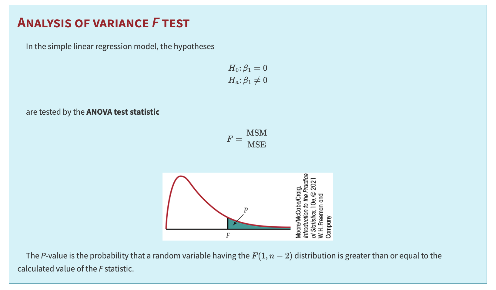
ANALYSIS OF VARIANCE \(F\) TEST

In regression, the hypotheses

\[H_0: \beta_1 = 0 \quad \text{vs.}\quad H_a: \beta_1 \ne 0\]

are tested with the ANOVA \(F\) statistic:

\[F = \frac{\text{MSM}}{\text{MSE}}.\]

The \(P\)-value is \(P(F(1, n - 2) \ge F_{\text{obs}})\).

The \(F\) statistic tests the same null as the \(t\) statistic. In fact, \(t^2 = F\). We often prefer the \(t\)-form in single-predictor regression for simplicity, especially for one-sided tests and confidence intervals.

12.5. Standard Errors

Inference for Slope and Intercept

Confidence intervals and significance tests for the slope \(\beta_1\) and intercept \(\beta_0\) of the population regression line use the estimates \(b_1\) and \(b_0\) and their standard errors. Some algebra and variance rules show that the standard deviation of \(b_1\) is:

\[\sigma_{b_1} = \frac{\sigma}{\sqrt{\sum (x_i - \bar{x})^2}}.\]

Similarly, the standard deviation of \(b_0\) is:

\[\sigma_{b_0} = \sigma \,\sqrt{\,\frac{1}{n} \;+\; \frac{\bar{x}^2}{\sum (x_i - \bar{x})^2}\,}.\]

We estimate these by replacing \(\sigma\) with \(s\).

STANDARD ERRORS FOR ESTIMATED REGRESSION COEFFICIENTS

The standard error of the slope \(b_1\) of the least-squares regression line is:

\[\text{SE}_{b_1} = \frac{s}{\sqrt{\sum (x_i - \bar{x})^2}}.\]

The standard error of the intercept \(b_0\) is:

\[\text{SE}_{b_0} = s \,\sqrt{\,\frac{1}{n} \;+\; \frac{\bar{x}^2}{\sum (x_i - \bar{x})^2}\,}.\]

Confidence Intervals and Prediction Intervals

When we substitute a particular value \(x^*\) of the explanatory variable into the regression equation and obtain \(\hat{y}\), there are two interpretations:

1. Estimate the mean response \(\mu_y\) at \(x = x^*\).

2. Predict a future observation \(y\) at \(x = x^*\).

Prediction intervals are broader than confidence intervals for a mean. Both depend on \(s\), the standard deviation about the fitted line.

STANDARD ERRORS FOR \(\hat{\mu}\) AND \(\hat{y}\)

The standard error of \(\hat{\mu}\) is:

\[\text{SE}_{\hat{\mu}} = s \,\sqrt{\,\frac{1}{n} \;+\; \frac{(x^* - \bar{x})^2}{\sum (x_i - \bar{x})^2}\,}.\]

The standard error for predicting an individual response \(\hat{y}\) is:

\[\text{SE}_{\hat{y}} = s \,\sqrt{\,1 \;+\; \frac{1}{n} \;+\; \frac{(x^* - \bar{x})^2}{\sum (x_i - \bar{x})^2}\,}.\]

The only difference is the extra “1” inside the square root for the prediction standard error, which accounts for the additional variation of individual responses around the mean.

Inference for Correlation

The correlation coefficient measures the strength and direction of linear association between two variables. We estimate the population correlation \(\rho\) using the sample correlation \(r\).

• If \(\rho = 0\), there is no linear association.

• If \(x\) and \(y\) are jointly Normal, \(\rho = 0\) also implies \(x\) and \(y\) are independent.

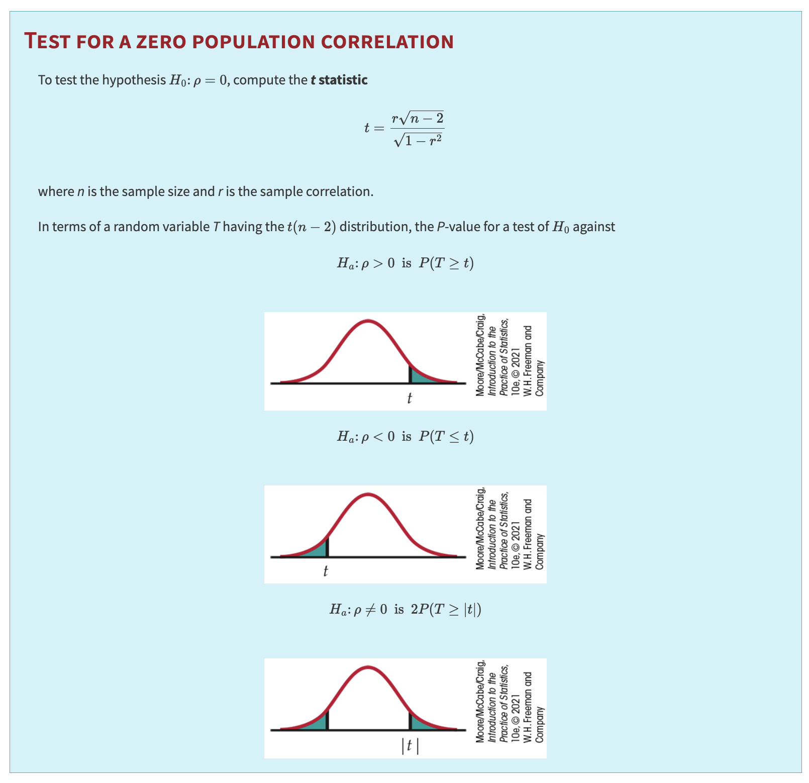
Test for a Zero Population Correlation:

To test \(H_0: \rho = 0\), compute the \(t\) statistic:

\[t = \frac{r \,\sqrt{\,n - 2\,}}{\sqrt{\,1 - r^2\,}},\]

where \(n\) is the sample size. The \(P\)-value depends on the alternative:

\[\begin{split}\begin{aligned} H_a\!: \rho > 0 & \quad\Rightarrow\quad P(T \ge t), \\ H_a\!: \rho < 0 & \quad\Rightarrow\quad P(T \le t), \\ H_a\!: \rho \ne 0 & \quad\Rightarrow\quad 2\,P(T \ge |t|). \end{aligned}\end{split}\]

TEST FOR ZERO CORRELATION

If \(T\) has a \(t(n - 2)\) distribution, then the \(P\)-value is found by comparing \(|t|\) to that distribution.

12.6. More details on standard errors of mean response and prediction

(12.1)\[y_i = \beta_0 + \beta_1 x_i + \varepsilon_i \quad\text{where}\quad \varepsilon_i \sim \mathcal{N}(0,\sigma^2).\]

Under OLS estimates, \(\hat{\beta}_0\) and \(\hat{\beta}_1\) have the following properties in simple linear regression (one predictor):

• \( \mathrm{Var}(\hat{\beta}_1) = \dfrac{\sigma^2}{\sum_{i=1}^n (x_i - \overline{x})^2},\)

• \( \mathrm{Var}(\hat{\beta}_0) = \sigma^2 \left[\dfrac{1}{n} + \dfrac{\overline{x}^2}{\sum_{i=1}^n (x_i - \overline{x})^2}\right],\)

• \( \mathrm{Cov}(\hat{\beta}_0,\hat{\beta}_1) = -\,\overline{x}\,\dfrac{\sigma^2}{\sum_{i=1}^n (x_i - \overline{x})^2}.\)

For any new point \(x_0\), the fitted mean response is

(12.2)\[\hat{\mu}_{y_0} \;=\; \hat{\beta}_0 \;+\; \hat{\beta}_1 \, x_0.\]

12.6.1. Deriving \( \mathrm{Var}(\hat{\mu}_{y_0}) \)

(12.3)\[\begin{split}\begin{aligned} \mathrm{Var}(\hat{\mu}_{y_0}) &= \mathrm{Var}(\hat{\beta}_0 + x_0\,\hat{\beta}_1) \\ &= \mathrm{Var}(\hat{\beta}_0) + x_0^2\,\mathrm{Var}(\hat{\beta}_1) + 2\,x_0\,\mathrm{Cov}(\hat{\beta}_0,\hat{\beta}_1). \end{aligned}\end{split}\]

Plugging in the standard results from above:

(12.4)\[\begin{split}\begin{aligned} \mathrm{Var}(\hat{\mu}_{y_0}) &= \sigma^2 \left[\frac{1}{n} + \frac{\overline{x}^2}{\sum (x_i - \overline{x})^2}\right] \;+\; x_0^2\; \sigma^2\!\biggl/\!\sum (x_i - \overline{x})^2 \;+\; 2\,x_0 \Bigl(-\,\overline{x}\,\dfrac{\sigma^2}{\sum (x_i - \overline{x})^2}\Bigr) \\ &= \sigma^2 \left[ \frac{1}{n} \;+\; \frac{(x_0 - \overline{x})^2}{\sum (x_i - \overline{x})^2} \right]. \end{aligned}\end{split}\]

Typically, we do not know \(\sigma^2\); we replace it by \(\mathrm{MSE}\), the mean squared error estimate from the regression. Thus,

(12.5)\[\mathrm{Var}(\hat{\mu}_{y_0}) \;=\; \mathrm{MSE} \left[ \frac{1}{n} \;+\; \frac{(x_0 - \overline{x})^2}{\sum_{i=1}^n (x_i - \overline{x})^2} \right].\]

Hence, the standard error of the estimated mean response at \(x_0\) is

(12.6)\[\mathrm{SE}_{\hat{\mu}_y} \;=\; \sqrt{ \mathrm{Var}(\hat{\mu}_{y_0}) } \;=\; \sqrt{ \mathrm{MSE} \left[ \frac{1}{n} \;+\; \frac{(x_0 - \overline{x})^2}{\sum_{i=1}^n (x_i - \overline{x})^2} \right] }.\]

12.6.2. Future Observation (Prediction Interval)

When predicting a future \(y\) at \(x_0\) — call it \(\hat{y}_0\) — we add in the irreducible noise \(\sigma^2\) from the new observation itself. In other words:

(12.7)\[\mathrm{Var}(\hat{y}_0) \;=\; \mathrm{MSE} \Bigl[ 1 \;+\; \frac{1}{n} \;+\; \frac{(x_0 - \overline{x})^2}{\sum_{i=1}^n (x_i - \overline{x})^2} \Bigr].\]

Thus the standard error for a future observation (used in a prediction interval) is

(12.8)\[\mathrm{SE}_{\hat{y}} \;=\; \sqrt{\mathrm{Var}(\hat{y}_0)} \;=\; \sqrt{ \mathrm{MSE} \left[ 1 \;+\; \frac{1}{n} \;+\; \frac{(x_0 - \overline{x})^2}{\sum_{i=1}^n (x_i - \overline{x})^2} \right] }.\]

---

[1]

In frequentist inference, we consider the parameters as fixed (but unknown) quantities, and the data as random due to sampling variability. In Bayesian inference, we treat the parameters as random variables with their own distributions (priors), and once the data is observed, it is considered fixed while we update our beliefs about the parameters through the posterior distribution.