
3. Chapter 3: Producing Data#
Since we have learned the concepts of population and sample, you might wonder how data is obtained for the population and sample. In the height example, we randomly drew a specific number of students from all Purdue students to form a sample. This gives us an abstract idea of the process of forming a sample. The concept of randomly drawing will be discussed in more detail shortly. However, let’s first focus on the population.
We can model the real-world measurements-the heights of all Purdue students-as a normal random variable, \(Height\), with parameters mean \(\mu\) and standard deviation \(\sigma\). This serves as a mathematical abstraction of the real-world phenomenon. This powerful abstraction allows us to quantify uncertainty, derive probabilities for outcomes, and perform statistical inference.
The randomness in height/\(Height\) may arise from many small factors, such as genetics, nutrition, environment, and other influences in biological or physical systems. Each observed height value is a realized outcome, or realization, of this process at the macro level. Modeling this process with a normal distribution is appropriate and can be explained by a fundamental concept, the Central Limit Theorem (CLT). Other processes and phenomena, however, may be modeled by different types of random variables.
Now, let’s turn our focus to sample data. The term parameter is associated with the population and is usually unknown. Once we have the sample data, we can follow a statistical procedure to calculate a STATISTIC, which is a number that describes the sample-for example, the sample mean.
Definition 3.1 (Statistic)
A numerical summary of a sample is called a statistic. The value of a statistic is known once we have taken a sample, but it can vary from sample to sample. Statistics are often used to estimate unknown parameters.
The entire process can be generalized as follows: First, we have a phenomenon that generates data. We model it as a random process with parameters. Next, we randomly draw or obtain data from the population to form our sample. From the sample, we calculate statistics, which we use to infer the parameters and thereby gain a better understanding of the random process and the real-world phenomenon.
This process can also be viewed as a generalization-using information from the sample to draw conclusions about the phenomenon.
3.1. Sources of Data#
Let’s explore the gap between the population and the sample. In the textbook, this leads to the question of sources of data. Whether we are interested in estimating the parameters of our population or making a conclusion about it, our questions of interest are inherently related to the population. However, we can only collect data from the sample.
This raises a fundamental question: Is our sample a good representation of the population of interest? If the sample is not representative, what we observe in the sample might not reflect the reality of the population. This is why the process of how we randomly draw or obtain the sample is critical to the entire process.
The term “sources of data” refers to the methods or origins of obtaining our sample data.
ANECDOTAL DATA and AVAILABLE DATA are two sources of data that we do not intentionally collect. These data sources might include only a few data points in the sample, and we usually lack full knowledge of how they were obtained. Therefore, we should be very cautious when drawing conclusions from these types of data.
Anecdotal data represent individual cases that often catch our attention because they are striking or unusual in some way. These cases are not necessarily representative of any larger group.
Available data are data produced for purposes other than our current question of interest but may still provide some insights or help answer the question.
To answer our questions of interest or draw conclusions about the population, it is usually better to create new data and form our sample intentionally. This critical step is often controlled by researchers to ensure the sample is representative and suitable for analysis.
There are two main approaches to obtaining data: one is through observational studies, often conducted via sample surveys[1], and the other is through experimental studies, conducted via experiments[2].
Definition 3.2 (Observational Study)
In an observational study, we observe individuals and measure variables of interest but do not attempt to influence the responses. Measure variables as they naturally occur (no intervention).
Definition 3.3 (Experiment)
In an experiment, we deliberately impose some condition or treatment (called an intervention) on individuals and we observe their responses.
3.2. Causality and Confounding#
When our goal is to understand cause and effect (causality), experiments are the only source of fully convincing data. The invention of randomized experiments was a stroke of genius; even today, they remain the gold standard for large pharmaceutical companies testing the effectiveness of new drugs.
This is because an observational study, even one based on a carefully chosen sample, is a poor way to determine what will happen if we change something. The best way to observe the effects of a change is through an intervention-where we actively impose the change.
The reason observational studies are a poor method for establishing causality is because of confounding. To establish a causal relationship, we typically aim to understand the relationship between an explanatory variable (or several) and a response variable.
For example, if we are investigating whether A causes B, A is the explanatory variable, and B is the response variable.
Definition 3.4 (Explanatory Variable)
An explanatory variable (sometimes called an independent variable, predictor, or factor) is the variable we think might explain or influence changes in another variable (the response variable).
In simpler terms, it’s the variable you suspect causes or predicts changes in the response variable (sometimes called the outcome or dependent variable).
Confounding occurs when an explanatory variable is related to one or more other variables (might be unobserved, hidden or lurking so you don’t have data for them) that also influence the response variable. These other variables are called confounding variables (or confounders). When confounding exists:
You may see an association between the explanatory variable and the response variable.
But some or all of that association might be due to a confounder that is linked to both.
Confounding can lead us to overstate or even mistakenly conclude that the explanatory variable caused the change in the response, when in reality, a confounding variable plays a partial or even dominant role in explaining that change.
For example, another variable, C, might cause both A and B. However, based on the observed data, you might incorrectly conclude that A causes B.
In an experiment, researchers actively impose an intervention (treatment) and use random assignment to decide who receives it. That way, any other factors that might affect the outcome (so-called lurking variables or confounders) should, on average, balance out across the different treatment groups. In an observational study, you are not assigning who or the subject is exposed to the treatment which might leads the confounding issue.
Two real life examples of confounding issues are:
The tobacco industry argued that a genetic variable, which could not be measured in the past, caused both smoking and lung cancer.
There is a strong correlation between a country’s annual per capita chocolate consumption and the number of Nobel Laureates per 10 million people.
Remember!
Association does not mean causation!
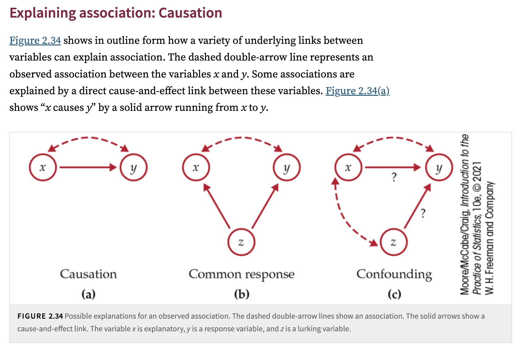
Fig. 3.1 Association and Causation#
3.3. Sampling Design#
Now that we have addressed the obstacles of confounding and understand why creating new data through experiments is sometimes necessary, we can revisit the critical step of getting our samples. Both observational studies and experimental studies require a well-thought-out sampling design. This is because we need to intentionally select elements or observations from the population to form a sample-a subset of the population-so that we maintain control over this step.
Unlike experimental studies, observational studies do not involve experimental design, which will be discussed in a later section. In observational studies, no treatments or interventions are deliberately imposed on the subjects. Instead, these studies rely entirely on sampling design to collect data. We will begin with a discussion of Sample Surveys, a classical form of observational study.
Definition 3.5 (Sample Survey)
A sample survey is an observational study-we simply observe, measure, or ask questions of a subset without imposing a treatment (as in an experiment).
The design of a sample survey refers to how we select the sample from the population.
The primary goal of sampling design is to ensure that the sample is selected in a way that guarantees it is representative of the entire population. If the sampling scheme favors certain parts of the population over others, it introduces bias, or systematic error.
One example of such a scheme is a voluntary response sample, where people who take the effort to respond to an open invitation are not representative of the entire population. This introduces a form of selection bias.
A voluntary response sample consists of people who choose themselves by responding to a general appeal. Voluntary response samples are biased because people with strong opinions, especially negative opinions, are most likely to respond.
Random selection of a sample eliminates bias by giving all individuals an equal chance to be chosen. This leads to Simple Random Sample (SRS) which is the most basic form of probability sampling. A probability sampling design uses a known chance (not necessarily equal) to select the sample.
Definition 3.6 (Simple Random Sample SRS)
Definition: Every set of \(n\) individuals in the population has an equal chance to be chosen.
Example: Names in a hat or using random digits/software to pick which individuals appear in the sample.
Here are two more complex sampling methods:
Stratified Random Sample: First, divide the population into strata (groups of similar individuals-e.g., by region, gender, or age). Then choose an SRS within each stratum and combine these SRSs into one overall sample.
Why? If individuals within each stratum are more alike, sampling each stratum separately can give more precise estimates (less variability).
It’s like blocking in experiments: grouping by an important characteristic before randomizing.
Multistage Random Sample (Including Clusters): Select the sample in stages. Common in large-scale national surveys:
Divide the population into primary sampling units (PSUs) (e.g., regions). Randomly select some PSUs.
Within each chosen PSU, randomly select smaller sub-units (e.g., city blocks).
Within each block, randomly select households or individuals (clusters).
Why? More practical (less travel and cost); large populations are spread out; a simple SRS of all households in the country would be logistically expensive.
Even with well-designed sampling methods, we cannot entirely eliminate bias. Below is a list of common sources of bias and errors.
Undercoverage: Some groups in the population are left out of the process (e.g., homeless, dorm students in telephone polls).
Nonresponse: Individuals chosen for the sample can’t be contacted or refuse to cooperate (often 50%+ in phone polls).
Response Bias: Behaviors of interviewer or respondent can influence answers (e.g., lying about sensitive topics, interviewer’s tone, memory errors).
Wording of Questions: Minor changes in phrasing can drastically change results. Leading or confusing questions create strong bias.
Measurement Bias: When your measurement process systematically mismeasures the target, consistently favoring one direction (e.g., a scale that overestimates weight).
One last thing I want to mention in this section is that our goal is to calculate a statistic[3] from our sample to estimate the parameter associated with the population. If the sampling design contains bias, you can imagine that this statistic will not be of high quality. However, bias is just one dimension when assessing quality. Another critical dimension is the variance, or variation, of a statistic during the sampling process, even if the sampling design is unbiased. Below are two common sources of variation.
Sampling Variability: If the sample is drawn from the population with some amount of randomness, the sampling variability describes the variability from one sample to the next.
Measurement Variability: When we take multiple measurements on the same object and we get variations in measurements from one sample to the next.
3.4. Design of Experiments#
Before diving into the design aspect, we first need to understand the definition of an experiment and familiarize ourselves with some terminologies associated with it.
Note
Experiment: A study in which researchers impose treatments (or interventions) on experimental units (which can be people, animals, or objects) in order to observe their responses (outcomes).
Why We Do Experiments: They’re our best shot at establishing cause-and-effect because by randomly assigning treatments and controlling conditions, we can reduce or eliminate confounding influences that otherwise might bias our conclusions.
Experimental units: The individuals in an experiment (called subjects if they are human). The smallest unit to which a treatment is independently assigned.
Factors: The explanatory variables in an experiment.
Example: A factor could be “Type of Class” (small vs. regular) in an education experiment, or “Ad Length” in an advertising study.
Outcomes (Response variables): The measured results (what we compare across treatments).
Example: students’ grades in the education experiment.
Levels of a Factor: Different values that a factor can take (e.g., 30-second vs. 90-second ad).
Treatments: Specific experimental conditions imposed on the subjects. Often formed by combining specific levels of one or more factors.
Example: If Factor \(A = Ad Length\) (30s or 90s) and Factor \(B = Repetitions\) (1, 3, or 5 times), you have 2 \(\times\) 3 \(=\) 6 possible treatments.
Placebo effect, Control, Control Group, and Treatment Group
Before we move on to how to design an experiment, we first need to clearly understand why we design experiments. In the previous sections, we learned that confounding is a significant issue when attempting to establish causality. The best way to avoid confounding is by conducting a comparative experiment. The basic idea is to assign (according to a specific experimental design) the experimental units into different groups after selecting them to form our sample. Each group receives a different treatment, and the results are then compared.
There are many potential variables or factors that could explain or affect the causal relationship between the variables of interest and the response variable. Often, confounders—hidden or lurking variables—cannot be measured, or they are not our primary focus. Experimental design aims to mitigate or eliminate the effects of these variables. This is the core idea behind experimental design: we need to Control these effects.
Definition 3.7 (Control)
Control is about managing lurking variables or extraneous factors (variables not of primary interest) that could influence the response variable.
If these factors differ between treatment groups, they may confound the results, making it unclear whether the observed differences are due to the treatments or the lurking variables.
The goal of control is to keep these variables constant or balanced across treatment groups, so any observed differences in outcomes can be confidently attributed to the treatments.
We will discuss how to achieve Control later when we explore experimental design. Since experiments involve two or more groups, we need a group to serve as a benchmark so that the results of other groups can be compared against it. This group is usually called the Control Group and is often given a Placebo to account for the Placebo Effect.
Definition 3.8 (Placebo Effect)
The placebo effect occurs when individuals experience a change in their behavior, symptoms, or outcomes simply because they believe they are receiving a treatment, even if the treatment has no active ingredient or direct therapeutic effect.
This psychological or physiological response is not due to the treatment itself but rather to the individual’s expectation of improvement or belief that they are being helped.
Baseline for Comparison: The placebo effect can confound the results of an experiment. To accurately measure the effect of a real treatment, researchers need to isolate the treatment’s effect from the placebo effect. This is why placebos are often used as a benchmark or baseline in experiments.
By including a placebo group, researchers can control for the impact of participants’ expectations or beliefs about the treatment, ensuring that any observed effects in the treatment group are due to the treatment itself and not psychological factors. The placebo control group can be thought of as a treatment group that receives no treatment. The remaining groups are referred to as treatment groups, each receiving a specific treatment.
How Placebos Work in Experiments:
Participants are Divided:
Some participants receive the actual treatment (e.g., a drug with an active ingredient).
Others receive a placebo (e.g., a sugar pill, saline injection, or inert substance) that looks identical to the actual treatment but has no active effect.
Blind or Double-Blind Designs:
Single-Blind: Participants don’t know if they are receiving the real treatment or the placebo.
Double-Blind: Neither the participants nor the experimenters know which group is receiving the real treatment or placebo. This eliminates biases from both sides.
Comparison:
After the experiment, researchers compare the outcomes in the treatment group to those in the placebo group. If the treatment group shows a significantly better outcome than the placebo group, the effect can likely be attributed to the treatment itself.
Types of Experimental Designs
Completely Randomized Design (CRD)
All experimental units are randomly allocated among all treatments.
Can handle any number of treatments.
Example: The advertising example with 6 treatments (two factors, each at multiple levels) and 150 subjects, randomly assigning 25 subjects to each treatment.
Matched Pairs Design
Often used to compare just two treatments.
Subjects are arranged in pairs (e.g., same age, same gender) that are alike in ways that might affect the response. Then one subject in each pair gets treatment A, the other gets treatment B.
Variation is reduced because each pair is more similar than randomly chosen individuals.
Alternatively, the same subject can receive both treatments in random order (the subject is “paired with themselves”). This experiment is called a cross-over experiment.
Block Designs
A generalization of “matching” when we have larger groups of subjects who share certain characteristics.
We divide subjects into blocks (groups) based on some confounding factor, then randomly assign treatments within each block.
Example: If men and women might respond differently, we block by gender, then randomize within each gender block.
For all designs, random assignment is essential at some stage. To implement randomization, we can use tools such as computer software, a table of random digits, or other similar methods.
One important strategy to note is that we can first block certain factors and then randomly assign treatments to groups within each block to control for lurking variables. This approach follows the principle: control what you can, block what you cannot control (i.e., form blocks), and randomize to create comparable groups-provided you have the luxury of a relatively large sample size.
We block these factors because they are not the focus of the study and can be observed by the researchers.
Core Principles of Experimental Design
Comparison: Use at least two treatments (or a treatment vs. control) to prevent confounding influences. Control: Keep outside variables (lurking or extraneous factors) the same or accounted for, so differences in outcome can be attributed to the treatments rather than confounding.
Randomization: Assign subjects to treatments purely by chance so the groups are (on average) similar in all respects except for the treatment imposed.
Repetition (Replication): Use enough subjects (or replicate the procedure multiple times) to reduce chance variation in the results.
3.5. Cautions about Experimentation#
Though randomized comparative experiments (when done carefully and repeated in different contexts) provide the strongest evidence for causation and are often regarded as the gold standard, there are still important considerations to keep in mind when conducting experiments and interpreting the results.
Lack of Realism: The experimental setting might not reflect real-world conditions, limiting generalizability.
Ethical/Practical Constraints: Some random assignments may be unethical (e.g., harmful interventions) or logistically impossible.
Approval of an institutional review board is required for studies that involve humans or animals as subjects.
Human subjects must give informed consent if they are to participate in experiments.
Data on human subjects must be kept confidential.
External Validity: Even a well-designed experiment in one setting might not hold for different populations or environments.
Bias and Confounding: If not carefully controlled, design flaws can still let lurking variables confound results.